Background.
This page is written with the assumption that the reader has studied the following pages:LOW NOISE AMPLIFIERS. HOW TO OPTIMIZE AND MEASURE PERFORMANCE.
Comparing NF measurements
Including the sub-pages linked to on those locations.
This page is an attempt to find all possible sources of error and uncertainty and to estimate the uncertainties in the final results on noise figures.
Tested amplifiers in October 2012.
-
1) MGF1425old This is the LNA that I used for EME in
the time period 1993 to 2001. This amplifier has never been
modified or adjusted since it was built in 1993 and the FET has
never been replaced. This amplifier has some front end selectivity
and uses neutralization.
-
2) MGF1801 This amplifier was built around 1997. It uses a wideband
input with low losses and it is neutralized. It has indicated an NF of
about 0.5 dB at some amateur meeting. In 2012 trimmers were added to adjust
the current as well as voltage. As a result the NF became significantly lower.
-
3) MGF1425 This amplifier was measured at the 7th EME meeting in Bowie
(near Washington DC) in 1996.
It was not well screened at the time, but it showed very low values
at times when no RF was leaking into it. This amplifier is neutralized and
uses a low loss wideband input. In 2012 trimmers were added to allow
voltage and current adjustment. Proper shielding was also added.
-
4) ATF33143 Built in 2001. Neutralized. Trimmers for voltage and current
adjustment added in 2012.
-
5) 2xATF33143 Built in 2001. Two transistors in parallel.
Neutralized. Trimmers for voltage and current adjustment added in 2012.
-
6) ATF33143negimp Built in 2012 with the purpose of demonstrating
negative noise figures on standard NF meters.
This amplifier has positive feedback and provides a return loss of -6 dB.
(The reflected power is 4 times higher than the incident power.
-
7) FHX05FA/LG Built Aug 2012 and tuned for optimum NF with Linrad
as a NF meter.
-
8) NONE No amplifier, just a BNC female to BNC female adapter.
Measurement system October 2012.
Linrad was running with the SDR-IP at a bandwidth of 1.2 MHz. A +23 dBm Schottky diode mixer was connected to the input with a HP8657A as the LO at 130 MHz. In front of the mixer a filter with more than 60 dB attenuation on the mirror frequency 116 MHz was inserted to ensure that all the signal reaching the SDR-IP on 14 MHz originated in 144 MHz. Low noise amplifiers in front of the filter provide a system NF of 3.3 dB.The output of the LNA under test was connected to the measurement system and the input was connected to a -58 dB directional coupler. The other side of the directional coupler was connected to a dummy load designed to withstand boiling water and ice water. Another HP8657A was coupled into the LNA under test with -58 dB attenuation.
Linrad was used to compare the noise in 1.2 MHz bandwidth to the signal from the second HP8657A which was accurately measured in a narrow bandwidth (which was excluded from the wideband noise computation.
Why use a directional coupler?
In previous studies, the signal was sent through an attenuator which was set to 0 C (ice/water) and 100 C (boiling water.) Evaluations were made assuming that the attenuation does not change with temperature. That is an approximation however, the attenuator used actually changed its attenuation by about 0.01 dB as measured on a network analyzer. The impedance change was 1.4% so there is an uncertainty due to the change of mismatch attenuation changes. The network analyzer is not exactly 50 ohms. The effect of the temperature variations of the dummy load on the obtained NF results are unknown, but not very large.By use of a directional coupler rather than an attenuator one can eliminate the effect of impedance variation with temperature.
Here is the place for the mathematics in case someone is interested to supply me with the proper formulae.
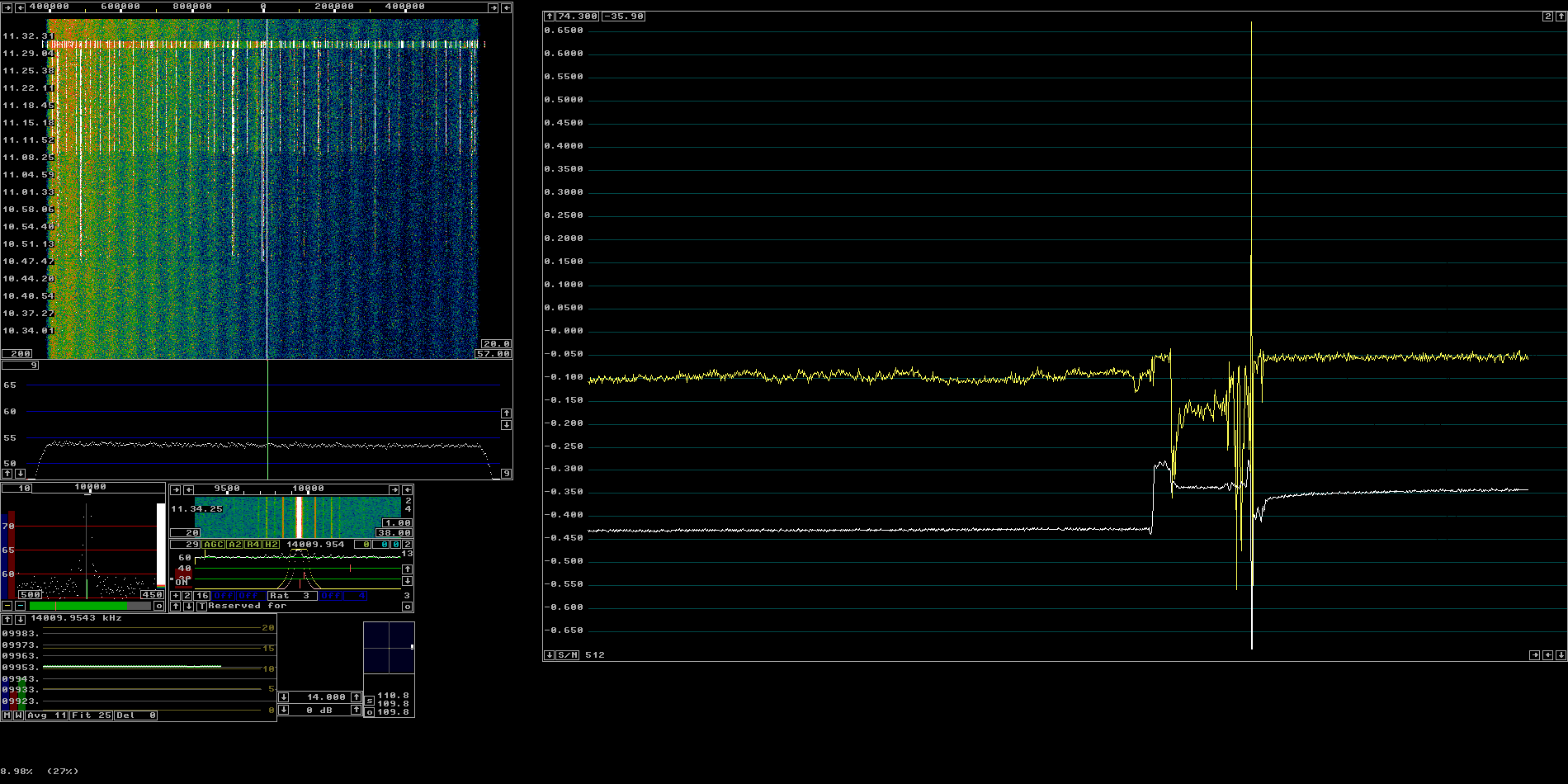
As a demonstration an impedance shifter, a LC circuit with 0.125 wl of cable after it was inserted immediately in front of the directional coupler. In figures 1 and 2 the S/N ratio (NF) and the signal level is shown for 50 ohms and impedance variations by about +/- 10% resistive and reactive.

| |||||||||||||||||||||||||||||||||||||||||||||||||||||||||||||||||||
| Figure 1. Real part of source impedance changed by +/- 10%. Actual impedance values at the input of the directional coupler were (54.4-j4.0) (50.2-j4.1) and (44.9-3.6j) | |||||||||||||||||||||||||||||||||||||||||||||||||||||||||||||||||
| |||||||||||||||||||||||||||||||||||||||||||||||||||||||||||||
| Figure 2. Imaginary part of source impedance changed by about +/- 5 ohms. Actual impedance values at the input of the directional coupler were (46.1-j1.5) (46.8+,2.1) and (47.9+j7.2) | |||||||||||||||||||||||||||||||||||||||||||||||||||||||||||
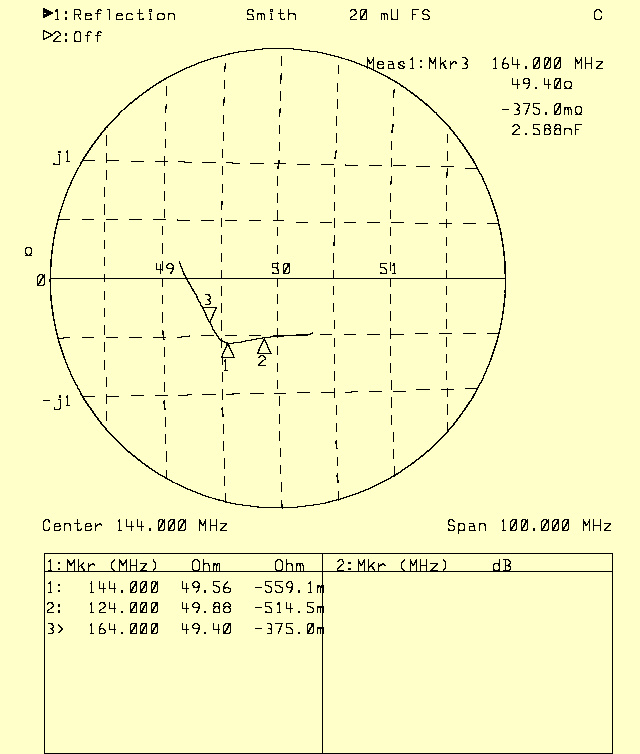
As can be seen from figures 1 and 2, the S/N ratio (yellow) changes by less than 0.03 dB for a 10% impedance change while the signal level (white) changes by as much as 0.35 dB. The room temperature impedance of the dummy load is (50.5+j1.5) at 144 MHz. Figure 3 shows the impedance change when going from 0 C to 100 C. The network analyzer was calibrated against the dummy load in ice/water and the Shmit chart was recorded with it in vividly boiling water. | |||||||||||||||||||||||||||||||||||||||||||||||||||||||||
| |||||||||||||||||||||||||||||||||||||||||||||||||||||||
| Figure 3. The impedance change from 0 to 100 C. Calibration was at C and the measurement at 100 C. | |||||||||||||||||||||||||||||||||||||||||||||||||||||
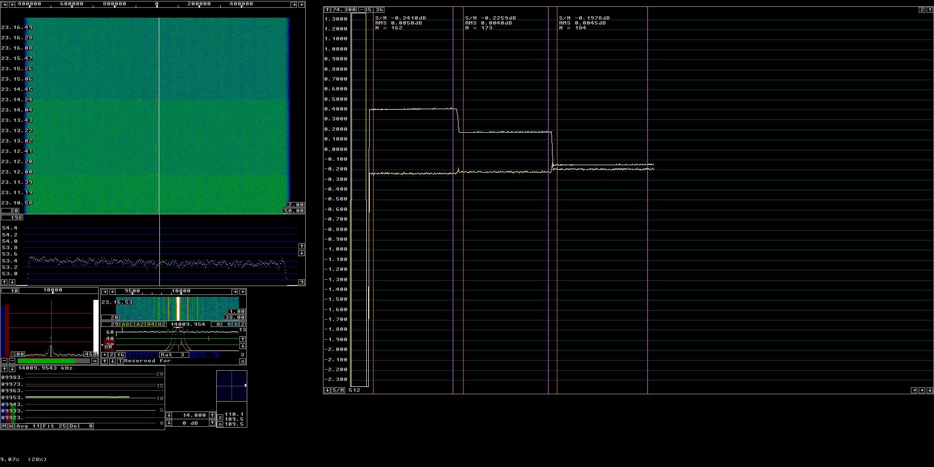
The impedance change due to temperature is about 0.7 ohms. Since the observed S/N changes by less than 0.03 dB for a 7 times larger change at the most, it should be safe to assume that the error due to temperature changes is less than 0.005 dB. Comments welcome. Particularly some math that would tell what to expect. Connectors.One of the major problems in precision measurements is contact resistance in connectors. N-connectors, and BNC connectors have the same problem in that the contact pressure is too low. With these connectors one should bend the outer fingers, ground on the male contact for an outer diameter that is 0.5 mm larger than the original diameter. The inner contacts should be gold plated. Whether to bend them to increase contact pressure or not depencs on the quality of the connector. Usually it is a good idea.Figure 4 shows a measurement of S/N where something is wrong. The main waterfall looks good from 10.30 to 10.50. Then something happens and the S/N is a little degraded. I had moved the LNA under test a little. At 11.09 things get worse. I moved the just a little more. At about 11.30 things become really bad. Note that the colour scale gain is 20 dB and each waterfall line is the average of 200 spectra. With normal settings one would not see this interference. The S/N graph shows an unstable noise flor at -0.1 dB. Then there is a short period of good noise floor at -0.05dB. Then S/N falls to -0.17 dB while the interference is strong. This means that the NF would be wrong by about 0.12 dB if measurements would be made with this interference present. The last part of the S/N graph shows a stable S/N at -0.05 dB. The error demonstrated in figure 4 was traced to inadequat contact pressure in a N-connector with golden center pin. Some bending and everything is stable when moving the cable. To get a stable system it is a good idea to bend all connectors. | |||||||||||||||||||||||||||||||||||||||||||||||||||
| |||||||||||||||||||||||||||||||||||||||||||||||||
| Figure 4. Poor contact pressure in a N-connector. See text. | |||||||||||||||||||||||||||||||||||||||||||||||
As a test on a precision NF meter with Linrad, move all cables and boxes around and look at the signal level as well as the S/N ratio. They should both be totally stable all the time. Crimp connectors are unreliable. I am very well aware that professionals say they are more reliable than connectors that have to be soldered. I have had several occurances of poor contact in professionally crimped connectors. Professionally soldered ones are not necessarily any better, but for ones own use one can take the time to do the work well. If you want to do precision measurements, use doubly screened cable and mount the connectors very carefully. Signal levels.There are several criteria for the signal levels. Linrad evaluates (Sb+Nb) which is the total power that passes the baseband filter and relates it to Nw) which is the power in the entire bandwidth supplied by the SDR-IP with an exception for a notch placed on the signal. For the computed S/N in the Linrad S-meter graph to be accurate to within 0.001 dB the S/N ratio in the baseband has to be above 36 dB and the contribution to the wideband noise from the HP8657A has to be 40 dB below the noise from the LNA under test.A test with LNA gain = 0 dB, the test system itself shows that the signal has to be in the range -44 to -15 dBm. That is with a baseband bandwidth of 2 kHz. When a low noise amplifier with 32 dB gain is under test the noise floor will be about 30 dB higher and therefore the signal level has to be in the range -14 to +15 dBm for the noise criteria to be fullfilled at a bandwidth of 2 kHz. There is another limit however. With a test object having 32 dB gain the SDR-IP saturates at -12 dBm. It is necessary to use a narrower baseband bandwidth. With a 20 Hz bandwidth the baseband S/N should be in the range 36 to 56 dB. The ice/water temperature.There are three problems with the cold temperature:1) The temperature can get too high if there is not enough ice so the dummy load has liquid water and no ice under it. Heat is slowly leaking into the container from below and liquid water has a limited thermal conductivity. This could be fixed by stirring, but better is to use plenty of ice to make sure there is a thick layer of water/ice slurry in all directions from the dummy load. 2) If the pieces of ice are large, like normal ice cubes, and taken directly from the refrigerator, the internal temperature is something like -18 C. It takes a long time for the temperature on the surface of such ice cubes to reach 0 C at the points where such surfaces are in contact with the dummy load. To be really safe one should allow at least two hours for the ice cube and water mixture to settle. It is necessary to stir frequently for a while, otherwise the ice cubes freeze the water between them and create big blocks of ice with even much longer times to wait until equilibrium. Wrap the ice cubes in a suitable piece of textile and crush them to small ice piecesr. Then thermal stability is reached well within 15 minutes provided that stirring is used to prevent the cold ice to freeze the water between the individual grains. 3) If the water contains dissolved salts, or other substances the freezing point will be below 0 C. By use of destilled water this problem is eliminated. The effect is well known, but experiment is easier than trying to find data on the Internet. 4.2 g table salt (NaCl) per litre improves the S/N by 0.0056 dB. That corresponds to a temperature change of about 0.4 degrees. Destilled water (battery water) contains less than 20 mg/l dry substances so the error in the freezing point should be in the order of 0.002 degrees. The boiling water temperature.The temperature for equilibrium between water and water vapour depends strongly on the pressure. The pressure in water increases by about 1 hPa for each centimeter below the surface. The correct place is to use the steam above the surface while making sure that the surrounding gas is water vapour only.An experiment adding 10 g of ordinary table salt (NaCl) to 2 litres of boiling water did not show any change of the S/N reading. The boiling point is far less sensitive to dissolved salt than the freezing point. The temperature characteristics of the directional coupler.The coupler is adjusted for -40 dB on 1296 MHz and it gives -58 dB on 144 MHz. The coupling varies a little with the temperature. Keeping the temperature well within one degree while moving the dummy load between hot and cold should make the coupler error smaller than 0.001 dB.Measurement conditions.All measurements on this page were made on Sept 10 2012. This day with stable weather the air pressure was reported to be 1015 hPa here in Eskilstuna. The table in Handbook of Chemistry and Physics, 1975-1976 gives the temperature of boiling water for pressures in mm Hg. 1015 hPa converts to 761.3 mmHg. My lab is 15 meters above sea level so the pressure in my lab should be 759.9 mm Hg. The handbook tells me that pure water would boil at 99.996 C. For the experiment "battery water" was used. It is demineralized water with a conductivity of less than 5 uS/cm. This water should be pure enough to boil and freeze at the expected temperatures 0.000 C and 99.996 C which convert to 273.15 K and 373.146 K.Raw data.The raw data listed in table 1 is obtained from the screen dumpsUnit S/N(0 C) S Gain Y-factor name (dB) (dB) (dB) (dB) ATF33143negimp -0.1934 60.0 32.1 1.2869 ATF33143 -0.2487 56.0 28.1 1.2697 FHX05FA/LG -0.1879 57.4 29.5 1.2794 MGF1425 -0.2636 58.4 30.5 1.2699 MGF1801 -0.2926 54.7 26.8 1.2580 2xATF33143 -0.3277 55.8 27.9 1.2536 MGF1425old -0.4698 59.1 31.2 1.2023 NONE -3.8642 27.9 0.0 0.6063Table 1.. | |||||||||||||||||||||||||||||||||||||||||||||
Evaluation.The total noise is the sum of the thermal noise of the dummy load, the noise from the tested amplifier and the noise from subsequent stages in the system 2nd Tinp. The Y-factor is the ratio of two such sums like this:Y = (373.146 + TLNA + 2nd Tinp)/(273.150 + TLNA + 2nd Tinp) | |||||||||||||||||||||||||||||||||||||||||||
   Unit         Y-factor Y-factor   Gain   2nd Tinp  TLNA    NF    NFEME2012   NFprev   Diff2012  Diffprev
  (name)         (dB)    (lin.pow)  (dB)    (K)     (K)    (dB)     (dB)     (dB)    (dB)    (dB)
ATF33143negimp  1.2869    1.34490   32.8   0.207   16.571  0.241    0.19     0.18    0.051   0.061
FHX05FA/LG      1.2794    1.34258   34.1   0.153   18.588  0.270    0.24     0.20    0.030   0.070
MGF1425         1.2699    1.33965   30.8   0.328   20.931  0.303    0.24     0.27    0.063   0.033
ATF33143        1.2697    1.33958   27.4   0.394   20.926  0.303    0.21     0.19    0.093   0.113
MGF1801         1.2580    1.33598   28.0   0.717   23.758  0.342    0.25     0.27    0.092   0.072
2xATF33143      1.2536    1.33463   28.5   0.557   25.119  0.362    0.28     0.30    0.082   0.062
MGF1425old      1.2023    1.31869   31.2   0.299   40.323  0.565    0.51     0.57    0.055   0.015
NONE            0.6063    1.14982    0.0    394
Table 2.. The noise figures evaluated from table 1 and compared to previous hot/cold measurements and to measurements made at the EME 2012 meeting. Note that The NF values of this page are not compensated for cable losses in this table. | |||||||||||||||||||||||||||||||||||||||||
|
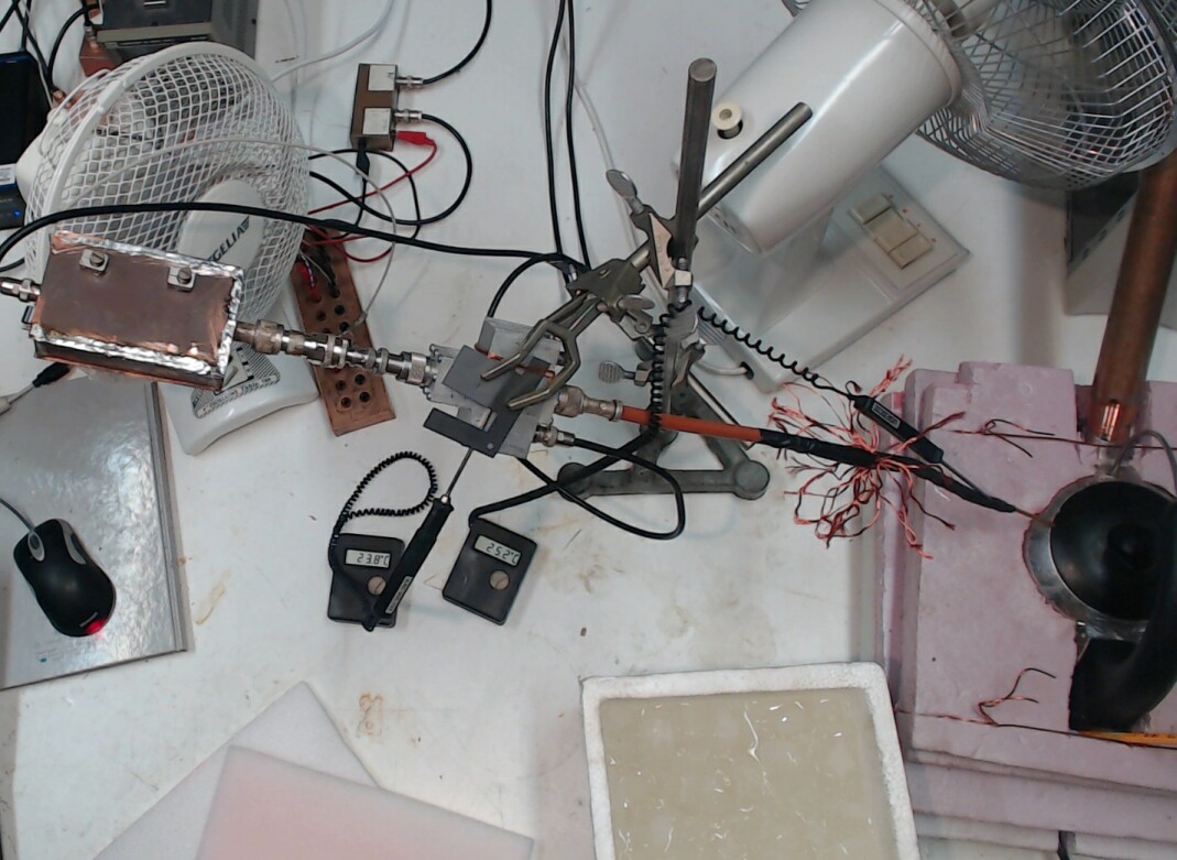
The cable from the dummy load to the test object is 290 mm of Suhner 02250 high temperature teflon cable. 90 mm of this cable is kept at (nearly) the same temperature as the dummy load and can be considered as part of the dummy load. 145 mm of this cable is kept near room temperature. That is accomplished by having about 50 square mm of litz wire twisted around the cable. There is also 230 mm of room temperature RG393. See figure 5. | |||||||||||||||||||||||||||||||||||||||
| |||||||||||||||||||||||||||||||||||||
| Figure 5. The dummy load in the steam of boiling water. The copper tube from the boiler is closed at the upper end. (It does not serve any purpose other than to close the boiler.) | |||||||||||||||||||||||||||||||||||
The temperature at the end of the litz wires was about 20 C when the dummy load was in the ice/water mixture and about 25 C when the dummy was placed in the steam of boiling water. The 55 mm of the cable over which the temperature changes from hot or colt to room temperature can be approximated as 30 mm of room temperature plus 25 mm of hot or cold. The nominal attenuation of Suhner 02250 is 0.33 dB/m so 175 mm should give a loss of 0.058 dB. The nominal attenuation of RG393 is around 0.078 dB/m so 230 mm of this cable should add 0.018 dB. The connectors and the directional coupler may add another 0.01 dB for a total of room temperature losses of 0.086 dB. | |||||||||||||||||||||||||||||||||
   Unit          NF    NFEME2012   NFprev   NFRel   Diff2012  Diffprev  DiffRel
  (name)        (dB)     (dB)     (dB)   (dB)    (dB)     (dB)     (dB)
ATF33143negimp  0.155    0.19    0.180   0.171  -0.035   -0.025   -0.016    -0.016   0.002   0.005
FHX05FA/LG      0.184    0.24    0.195   0.206  -0.056   -0.011   -0.022    -0.037   0.016  -0.001
MGF1425         0.217    0.24    0.271   0.232  -0.023   -0.054   -0.015    -0.004  -0.027   0.006
ATF33143        0.217    0.21    0.188   0.237   0.007    0.029   -0.020     0.026   0.056   0.001
MGF1801         0.256    0.25    0.267   0.270   0.006   -0.011   -0.014     0.025   0.016   0.007
2xATF33143      0.276    0.28    0.302   0.293  -0.004   -0.026   -0.017     0.015   0.001   0.004
MGF1425old      0.479    0.51    0.567   0.523  -0.031   -0.088   -0.044    -0.012  -0.061  -0.023
Average                                         -0.019   -0.027   -0.021      0.0     0.0     0.0
                                                                         RMS 0.022   0.034   0.010
Table 3.. Here the losses of the cables are included.
The noise figures from the study on this page are compared to measurements
made at the EME 2012 meeting.
and to previous hot/cold and relative NF measurements
| |||||||||||||||||||||||||||||||
|
Table 3 indicates that there was a systematic error of -0.027 dB in the previous hot/cold measurements using an attenuator. Presumably that would be due to the variation of the attenuation with temperature, at least in part. This error was transferred to the EME2012 results as an error in the correction for the noise head. Instead of 0.07 dB the correction should have been 0.05 dB. The thre last columns in table 3 are for computing the RMS deviation for the differences after having shifted the zero point of the respective NF columns by 0.019, 0.027 and 0.021 dB respectively. It is quite clear that the results on this page show a close agreement with the previous relative measurements while the previous hot/cold measurements were less accurate. It would have been interesting to compare with the results obtained with a circulator at the meeting, but unfortunately those results have not been made public. The measurements on this page were obtained at a room temperature of 23.8 C while the EME measurements were made at a somewhat higher temperature. The NF of GAAS FET amplifiers depend on the temperature. The FHX05FA/LG amplifier which has NF=0.18 dB at room temperature would have a NF of 0.28 dB when used at the mast top in the sunshine in Texas (70 degrees centigrade) while the same amplifier in Alaska at 30 degrees below the freezing point would have an NF of about 0.11 dB. On 144 MHz where I made these experiments it does not matter, but on higher bands it seems worthwhile to use Peltier coolers to improve the noise figure. Tested amplifiers in November 2012.
| |||||||||||||||||||||||||||||
Unit                IIP3    1dB sat.    Gain    OIP3
                   (dBm)     (dBm)      (dB)   (dBm)
MGF1425narrow       -11       -19       26.7    +16
MGF1801              -6       -17       26.1    +20
MGF1425november     -11       -20       25.3    +14
ATF33143             -9       -19       26.2    +17
FHX05FA/LGnovember  -10       -21       27.1    +17
NE334-S01           -15       -26       28.5    +14
PSA4-5043            +7        -5       23.8    +31
AD6IW                +4        -7       24.3    +28
Table 4.Third order intermodulation gain and the point of
1 dB compression for the amplifiers studied November 2012.
IP3 is measured for the input level that gives IM3 about 45 dB
below the two tones.
| |||||||||||||||||||||||||||
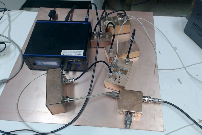
Measurement system November 2012.The RF hardware used for this set of measurements is shown in figure 6. | |||||||||||||||||||||||||
| |||||||||||||||||||||||
| Figure 6. The RF hardware used for measurements with Linrad in november 2012. | |||||||||||||||||||||
The RF hardware is improved since October. Everything is put on a conducting surface to reduce electric fields. The Ethernet cable from the SDR14 to the computer has a screen that now is connected to the chassis of the SDR-14. There are several ferrite tubes on the Ethernet cable but the screen is not connected to anything at the other end. The signal enters the SDR-14 through a BLP-15, a 15 MHz lowpass filter from Minicircuits. This filters eliminates some spurs that presumably are due to the 133 MHz LO and was not used in October. The cable to the BLP-15 filter comes from a box that contains a high level mixer, 23 dBm, from Minicircuits. The mixer is driven from a power amplifier that delivers 25 dBm LO power to the mixer. The high LO level saturates the mixer and makes conversion loss insensitive to the LO level. The RF port is connected through a filter that eliminates signals on the mirror frequency. (More than 60 dB attenuation.) The 144 MHz signal enters the filter from an identical amplifier as the one used for the LO. (This pair of amplifiers were designed for IM3 measurements.) The high level amplifier is fed from a GAAS-FET LNA, the 2xATF33143 unit with NF about 0.3 dB. To get a goodd load impedance for the test object a circulator is added in front of the LNA. This degrades the NF to about 1 dB. In october a BFR91 amplifier was used without circulator. ALL coaxial connectors have their outer contacts bent for higher than nominal contact pressure. This is a VERY important thing in the high interference level created by computers and screens only about 1 m away from the RF equipment. The circulator is covered with copper foil. It is not well enough screened in its original shape. All cables are doubly screened. Most of them are RG223. Hot/cold measurements Nov 18 2012.The hot/cold arrangement is the same as shown in figure 5 but the the thin cable between the dummy load and the room temperature cable has been thermally insulated starting 70 mm from the dummy load.Measurements were made in the evening at a time when the local weather forcast reported a stable air pressure of 1008.7 hPa for Eskilstuna. That corresponds to 756.6 mm Hg. Correcting for my location 15 m above sea level givet the pressure in my lab as 755.2 mm Hg. Handbook of Chemistry and Physics, 1975-1976 tells me that pure water boils at 99.82 �C. That is 372.97 K. The cold temperature is 273.15 K. The raw data and evaluation is displayed in table 5. Y-factors are from screens like the ones used for table 1. I did not save them this time. The Y-factor which comes directly from the measurement is equal to this expression: Y = (372.97 + TLNA + 2nd Tinp)/(273.15 + TLNA + 2nd Tinp) The Y-factor when NONE is the DUT gives the system noise figure at the connector on the BNC female to female adaptor. Then there is no 2nd T to take into account. The term 2nd Tinp becomes low because the system noise temperature at the connector is only 87.8 K. The gain is needed to compute the contribution of the system noise figure at the DUT output. The gain values are computed from the RMS power of the narrowband signal. The room temperature was 24 �C and the temperature at the end of the litz wires should stay at this temperature all the time since the cable is now thermally insulated. The 75 mm of the cable over which the temperature changes from hot or cold to room temperature can be approximated as 35 mm of room temperature plus 30 mm of hot or cold. The nominal attenuation of Suhner 02250 is 0.33 dB/m so 185 mm should give a loss of 0.061 dB. The nominal attenuation of RG393 is around 0.078 dB/m so 230 mm of this cable should add 0.018 dB. The connectors and the directional coupler may add another 0.01 dB for a total of room temperature losses of 0.089 dB. | |||||||||||||||||||
   Unit            Y-factor Y-factor   Gain   2nd Tinp  TLNA    NF    NFfinal
  (name)            (dB)    (lin.pow)  (dB)    (K)     (K)    (dB)     (dB)
MGF1425narrow      1.2453    1.33208   26.7   0.188   27.25   0.390    0.301
FHX05FA/LGnovember 1.2786    1.34233   27.1   0.171   18.27   0.265    0.176
NE334-S01          1.2900    1.34586   28.5   0.124   15.34   0.224    0.135
MGF1801            1.2490    1.33321   26.1   0.216   26.20   0.376    0.287
ATF33143           1.2543    1.33484   26.2   0.211   24.75   0.356    0.267
MGF1425november    1.2627    1.33743   25.3   0.259   22.41   0.323    0.234
ATF33143november   1.2845    1.34416   28.1   0.136   16.74   0.244    0.155
PSA4-5043          1.1648    1.30761   23.8   0.366   50.98   0.703    0.614
AD6IW              1.2009    1.31853   24.3   0.326   39.90   0.560    0.471
NONE               1.0603    1.27653    0.0     -     87.8    1.150    1.061
Table 5. Hot/cold results November 2012. | |||||||||||||||||
|
In total the MGF1801 and ATF33143 amplifiers have been measured with ice and steam three times. Two of them presented on this page, the third was Aug 13 2012 All the results are listed in table 6. | |||||||||||||||
   Unit             Aug      Oct    Nov     Average    RMS
MGF1801             0.267   0.256   0.287    0.270    0.013
ATF33143            0.188   0.217   0.267    0.224    0.032
Table 6.. The three sets of hot/cold measurements on the two amplifiers that have been left unchanged. | |||||||||||||
|
Table 6 indicates that the RMS error in an individual measurement with the hot/cold method might be 0.03 dB although the number of data points is far too small for any real conclusion. Each Y-factor is the difference of two noise power levels. Those pover levels are the average of a couple of hundred noise powers and the RMS deviation is typically 0.003 dB which would mean a statistical error of about 0.0002 dB but that would be true only if there is no drift in the system. It seems reasonable to assume that the errors in the two power levels are 0.01 dB which would mean that the RMS error in the Y-factor would be 0.015 dB. For a typical Y-factor like 1.25 dB, the Y-factor in linear power scale should then be in the range 1.3289 to 1.3381. If we assume that the temperature error is negligible we can solve the error limits from these equations for a typical ice/steam experiment: 1.3289 = (373 + TLNA )/(273 + TLNA ) 1.3381 = (373 + TLNA )/(273 + TLNA ) The two temperatures become 22.77 and 31.04 K and the corresponding NF values 0.33 and 0.44 dB or 0.385 �0.055 dB. It seems that the RMS error in the Y-factor when measuring a single move from hot to cold or vice versa is about 0.005 dB. with an RMS error on NF values of 0.025 dB. To improve it would be necessary to move many times between the two temperatures. That would make any drift visible and should allow a good knowledge of the error in the Y-factor. To move 10 times into each temperature it would be necessary to make a new dummy load with much smaller time constant. Measuring S/N at different bandwidths and temperatures.A room temperature dummy load was inserted between the signal generator and the test object and S/N was measured at different room temperatures and different bandwidths. The temperature affects the signal generator and the directional coupler but once the temperature is stable S/N levels are stable. Table 7 shows the observed S/N values. In S/N measurements one can only see the difference in NF between different amplifiers. For this reason all NF values are shifted by the same amount to make the average of the three wideband cases PSA4-5043, AD6IW and NONE equal to 0.7153. That is their average in table 5. | |||||||||||
Unit 24.6�C 24.6�C 24.6�C 29.5�C 11.2�C Average RMS Table 1 Diff
125kHz 500kHz 2MHz 500kHz 500kHz hot/cold
MGF1425narrow 0.322 0.356 0.308 0.339 0.335 0.332 0.016 0.301 0.031
FHX05FA/LGnovember 0.182 0.193 0.182 0.198 0.199 0.191 0.007 0.176 0.015
NE334-S01 0.137 0.144 0.136 0.151 0.157 0.145 0.008 0.135 0.010
MGF1801 0.275 0.287 0.278 0.292 0.294 0.285 0.008 0.287 0.002
ATF33143 0.238 0.255 0.245 0.256 0.246 0.248 0.007 0.267 0.019
MGF1425november 0.237 0.249 0.243 0.254 0.254 0.247 0.005 0.234 0.013
ATF33143november 0.152 0.167 0.170 0.166 0.169 0.165 0.007 0.155 0.010
PSA4-5043 0.609 0.624 0.626 0.618 0.630 0.621 0.007 0.614 0.007
AD6IW 0.455 0.467 0.472 0.470 0.457 0.464 0.008 0.471 0.007
NONE 1.082 1.056 1.048 1.058 1.060 1.060 0.011 1.061 0.001
Table 7.. Values in dB.
| |||||||||
|
Table 6 shows that the room temperature is not important for the NF differences between different amplifiers. That is not unexpected. The temperature change from 29.5 to 11.2 �C is 18.3 degrees should change ths NF by about 0.03 dB. The RMS deviation between the two columns for 11.2 and 29.5 �C is 0.07 which means that all the amplifiers are affected by the nearly the same amount. The value 1.082 for NONE at 24.6 �C/125kHz deviates significantly and is probably an error. MGF1425narrow has a too small bandwidth to be measured this way. If one tunes it for optimum NF at 2 MHz bandwidth one finds negative NF values because the noise is better suppressed with a looser coupling on the input that makes the bandwidth narrower at a modest increase in the NF. The unit was tuned at 300 kHz where the tuning error is reasonably small. The reasonable NF value at 2 MHz for MGF1425narrow is unexpected and probably just a coincidence. The differences between hot/cold values from table 1 and the averages of all five columns in table 7 have a RMS value of 0.011 dB. That is significantly larger than the average RMS deviations between the columns and indicates that the statistical errors in the hot/cold method is something like 50% larger than the errors in the S/N method. The best estimate for the NF of these amplifiers would then be as shown in table 8, Col 1, "weighted average Nov 21," where MGF1425narrow is excluded for its narrow bandwidth. The hot/cold is averaged with the average S/N result with a weight of 0.1 to form an average of six measurements where one is weighted by 50% because its error is twice as large. Another way of measuring relative noise figures is with standard instruments and circulators. Such studies were made at EME 2012 but not published when this page was written. The amplifiers listed in table 8 were tested with two different HP8970B noise figure meters and circulators. Four series of measurements were made on Nov 23 2012 detailed description and raw data is available here. The relative measurements have an average deviation from the "Weighted average Nov 21" of 3.600 dB. The data in table 8 is therefore the measured NF -3.60 dB. The purpose of table 8 is to compare it with NF results from measurements with standard NF meters using the 0.25 wl metod or using circulators. The "weighted averages Nov 21" are formed from 5.5 values with RMS deviations about 7. The RMS error in each of the weighted averages should then be expected to be sqrt(5.5) times smaller which is 0.003 dB. To this random error comes a much larger systematic error that is equal for all amplifiers. The tentative error analysis above suggests it comes from random errors in Y-factors. Six of them are used to set the zero point and if one assumes they have a RMS error of 0.03 dB the systematic error should be 0.013 dB RMS Applying the three sigma rule it would be appropriate to say that each NF value in table 7 has an error limit of 0.04 dB but the relative NF values are much more accurate. | |||||||
                    Col 1      Col 2     Col 3     Col 4   Col 5
   Unit            Weighted   8970B(1)  8970B(1)  8970B(1)  8970B(2)
                   average    2circ(1)  2circ(2)  1circ    2circ
                    Nov 21     Nov 23    Nov 23   Nov 23   Nov 23
FHX05FA/LGnovember  0.190       0.19      0.19     0.18     0.19
NE334-S01           0.144       0.14      0.14     0.14     0.14
MGF1801             0.285       0.28      0.29     0.29     0.29
ATF33143            0.250       0.24      0.25     0.25     0.25
MGF1425november     0.246       0.24      0.25     0.24     0.25
ATF33143november    0.164       0.16      0.16     0.16     0.17
PSA4-5043           0.620       0.61      0.61     0.64     0.63
AD6IW               0.465       0.47      0.47     0.47     0.47
Table 8.. NF values in dB.
| |||||
|
The four columns, columns 2 to 5 with data from Nov 23 have a maximum deviation of 0.02 dB from col 1 but only in one single place and that is in the column for measurement with a single circulator. Most deviations are smaller than 0.01 dB. Columns 2 to 5 show that comparisons of preamps using standard instruments with circulators have an accuracy of 0.01 dB. Probably better if modern instruments with builtin temperature sensors and readouts with more decimal places were used. The purpose of measuring relative NF with extreme accuracy is to allow the measurement of losses in adaptors, connectors, relays and other low loss components that may degrade the NF of real world systems. Those small losses can not be measured with network analyzers since there are also mismatch losses which are harmless for the NF but contribute to the losses we see on a network analyzer. It is of course helpful to be able to measure NF correctly with two decimals when optimizing amplifiers for frequencies with very low sky noise. Measurements with a modern NF meter.Measurements were done on December 28 2012 with a noise head N4000A and an Agilent 8973A noise figure meter. This was a joint effort by Mart, SM0ERR and myself, Leif, SM5BSZ. The results agree with the data described above better than expected. Table 9 shows the results in short. | |||
   Unit            Weighted    8973A       Diff
                   average     average
                    Nov 21     Dec 28
FHX05FA/LGnovember  0.190       0.1846    0.0054
NE334-S01           0.144       0.1420    0.0020
MGF1801             0.285       0.2874   -0.0024
ATF33143            0.250       0.2525   -0.0025
MGF1425november     0.246       0.2495   -0.0035
ATF33143november    0.164       0.1620   (0.0020 oscillates on circulator)
PSA4-5043           0.620       0.6191    0.0009
AD6IW               0.465       0.4731  (-0.0081 oscillates on circulator)
Table 9.. NF values in dB and differences between columns.
| |
The details of our measurements are presented here: details of NF measurements with N4000A and Agilent 8973A The N4000A gives a 0.025 dB lower NF than the hot/cold method with ice and steam did in November 2012. That is compensated for in table 9. The relative NF scales show a next to perfect agreement just as the data collected at the 2012 EME meeting by Dominiqe, HB9BBD does to an even higher degree. Agilent specifies the accuracy of the noise head calibration to be 0.16 dB in this frequency range. That seems like a very conservative specification in light of table 9. The N4000A is very good in that the impedance does not change much from cold to hot. The one we used changes by 0.30 ohms from off to on. With the cable loss properly accounted for, the NF reading for non-matched GAAS FET LNA typically differs by 0.05 dB depending on whether the quarterwave cable is inserted or not. This means that the error due to variations in the source impedance of the N4000A is only 0.025dB on the tested set of near infinite SWR amplifiers. With MMIC amplifiers the difference is one order of magnitude smaller. There could be systematic errors in the hot/cold measurements with ice and steam and the good agreement with the N4000A could be accidental. There is no question however that relative NF values can be determined well within 0.01 dB either by use of a circulator or by use of the average of two measurements with and without a 0.25 wl cable. |