Fig 1. Set the width over which the average pulse should be considered non-valid near the center on this screen.
About this page.The purpose of this page is to provide some understanding of the calibration procedure used in Linrad. This page demonstrates how to calibrate one particular hardware unit. The file containing calibration pulses can be downloaded and used to produce the calibration files dsp_xxx_corr that would work with this particular set of WSE units.Erase any dsp_xxx_corr file that may be present in your Linrad directory (or create a new Linrad directory without such files.) Download the files containing calibration pulses and go through the calibration procedure to become familiar with it. Finally erase the dsp_xxx_corr files. They are of no use with your own hardware even if it is a WSE converter. With the experience you will get it should be easier to perform the calibration on your own hardware. Hardware and raw data.The calibration pulses are contained in http://www.sm5bsz.com/linuxdsp/flat/cal2/blankerinit2.raw (50Hz, 6 341 753 bytes) To study the influence of the pulse repetition rate you might want to download one of these files http://www.sm5bsz.com/linuxdsp/flat/cal2/blankerinit4.raw (5Hz, 6 106 745 bytes) or http://www.sm5bsz.com/linuxdsp/flat/cal2/blankerinit5.raw (400Hz, 6 226 553 bytes). These file were recorded with the WSE converters and a Delta 44 soundcard. The calibration pulses is the square wave TTL output from a function generator (Escort EGC 2230) which was connected directly to the RXHFA input which was set to +10 dB gain at 3.6 MHz.To do the calibration procedure from one of the three files above, place the file in a directory /demo if you run under Linux or in a directory c:\demo if you run under Windows. Then place a file adfile or adfile.txt in the directory from where you launch Linrad. Use one of these files adfile for Linux or adfile.txt for Windows depending on the OS you are using. You also have to create a subdirectory par under demo. This is where Linrad will place the parameter files for this recording as specified in adfile. Running for the first timePress 3 to select one of the files you have in your demo directory. When running for the first time Linrad will prompt for the receive mode to use. Select any mode, i.e. Normal CW. You must then answer Y to the question Repeat recording endlessly because Linrad will read from the file at 96000 samples per second while you set filter parameters and Linrad will hang in the calibration routine if end of file is reached.Linrad will remember your choices in the file blnkini_2 under the par subdirectory under demo as specified in adwav. You will then be prompted for the mode parameters unless you already have calibration files for the WSE converters in the directory from where you launch Linrad. (If you have, it might be a good idea to save them and then remove the calibration files (dsp_xxx_corr) from your Linrad directory. The calibration procedure is described here: flat frequency response Collect the average pulse shape.Go to the collect averages screen, look here Calibration for two channels if you are not familiar to the Linrad menu system.The three files at 5, 50 and 400 Hz contain about 100, 1000 and 8000 pulses respectively and collecting each pulse more than one time is meaningless. Collecting for the duration of the file, about 10 seconds, will give a good enough S/N with a broad margin. Set the desired filter response.When U is pressed on the collect averages screen, you arrive at the screen for setting the desired filter response.The focus on this page is on the interpolation across the center discontinuity and you are assumed to already know about how to set the desired filter response so just press Y on this screen to return to the collect averages screen on which you should then press S followed by X to return to the menu from where you can again go to the calibration menu. Remove the center discontinuity.In a soundcard based direct conversion receiver there is an infinitely deep notch in the spectrum caused by the fact that soundcards are not DC coupled. When collecting calibration pulses, Linrad can not analyze a much longer time span than the time between two pulses and that causes another high pass filter on top of the one supplied by hardware. It will be present also with DC coupled hardware.Phase and amplitude determined from the average pulse will not be correct at the center frequency, but by interpolation across the center region Linrad can make sure that the curves on both sides of the notch match each other. The first screen of the remove center discontinuity procedure is shown (in part) in figure 1. With the blankerinit1.raw file, the default setting, 515 Hz is reasonable. A 50 Hz square wave gives pulses that repeat at 100 Hz and the flat region of the window used to select a single pulse corresponds to 200 Hz so excluding 2.5 times more bandwidth seems reasonable. | |

Fig 1. Set the width over which the average pulse should be considered non-valid near the center on this screen. | |
|
There are four screens to interpolate across the center discontinuity.
The curves are nearly symmetric or antisymmetric around the center frequency
and it is advantageous to use the symmetry properties.
The first interpolation across the center is converted to an extrapolation to zero (the midpoint) of the antisymmetric amplitude, figure 2. To understand what figure 2 shows, first look at figures 2A and 2B. | |

Fig 2A.The averaged pulse response as collected by the calibration routine. Green is phase and magenta is amplitude. It is obvious that the amplitude is close to symmetric. The left side is close to a mirror image of the right side. The spectrum is obtained from an I/Q pair that is obtained from a quadrature detector. Anti-alias filters as well as the center low pass filter (DC blocking) will affect audio exactly the same regardless of the phase relation between I and Q and therefore give an exactly symmetrical response. There is however also an RF filter at 2.5 MHz and the contributions from that is not quite symmetric. The phase curve is anti-symmetric. The left side is the negative of the right side. | |

Fig 2B.The center part of figure 2A with expanded scales. It is quite clear from this image that the 2.5 MHz filter is not quite symmetric. It is close to flat but has a little ripple with three peaks. The center peak of the 2.5 MHz filter is a little below 2.500 MHz. That produces the best over-all filter response. | |

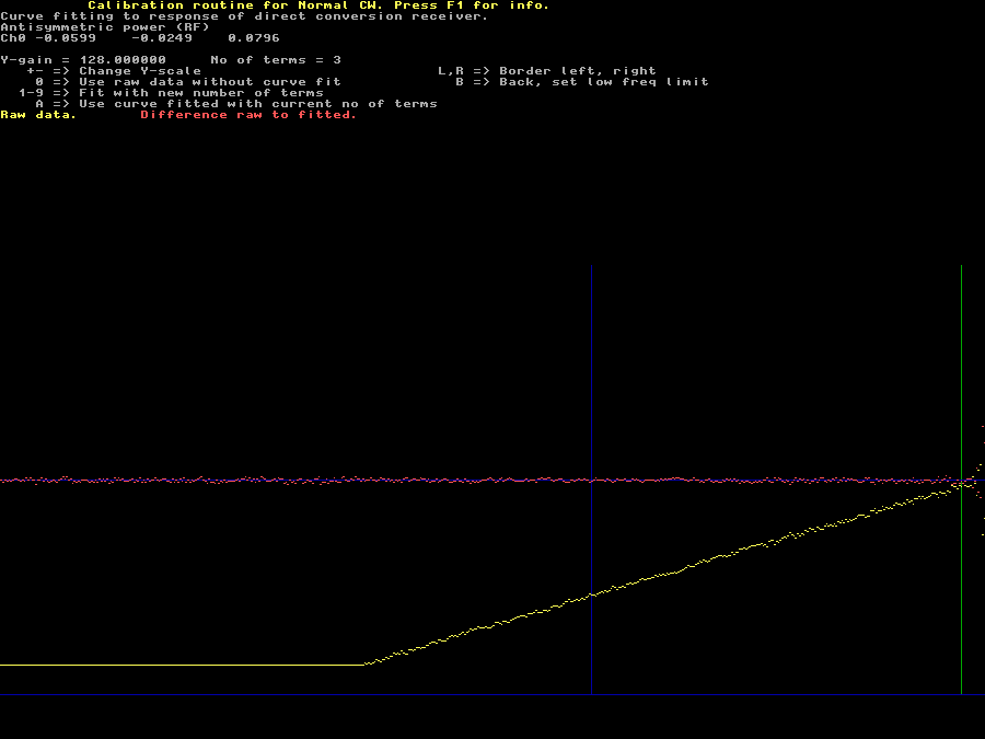
Fig 2. The anti-symmetric power, the yellow line, reflects the slope of the amplitude response of any RF filters in front of a direct conversion receiver. The yellow line is the difference between the green data points on either side of the center in figures 2A or 2B. This line must go to zero at the right hand side of the graph where the center point would be subtracted from itself and give a zero. The yellow line is very well represented by a third order polynomial: Y = - 0.0599 * X - 0.0249 * X2 + 0.0796 * X3 The red line is the difference between the polynomial and the measured data. Typing A to this screen means that the values computed by the polynomial will replace the experimental data at the right hand side of the blue line. In this case it does not matter where the blue line is placed. | |
|
It is obvious from figure 2 that the RF filters of the WSE converter chain
have an amplitude spectrum with a negligible second derivative across
the center discontinuity.
When a polynomial in 3 terms is fitted to the raw data, the yellow curve,
the difference raw data to fitted data is very close to zero except for about
half the excluded region of 515 Hz to the right.
Note that the vertical scale is expanded 128 times.
Using the polynomial will be very safe - and it will not matter
what number of terms one chooses for the curve fitting.
Just press A to use the polynomial rather than the (incorrect)
data points across the center notch.
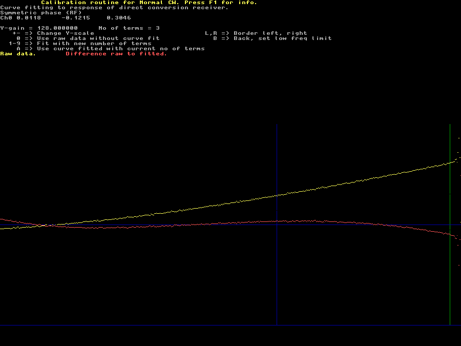
The next two screens are also straight-forward. The antisymmetric phase has a nonzero value for X=0 that corresponds to half the phase jump of the green curve at the center of figures 2A and 2B. It is very well reproduced by a 5 term polynomial. The symmetric power, the sum of the magenta points in 2A and 2B is also nonzero at X=0. It is well represented by a 4 term polynomial. From figure 2B we can see that the center region is close to a parabola but the third screen shows that one has to include a 3rd order term to get a good fit to measured data. The last screen, the symmetric phase that corresponds to the phase response of all the RF filters in front of the I/Q mixer is more difficult. See figures 3 and 4. | |

Fig 3. The symmetric phase reflects reflects the phase response of the RF section. It is the sum of the green points on either side of the center in figures 2A and 2B. It has higher order derivatives and needs many terms in the polynomial fit. Here the number of terms is 3. Compare with figure 4 | |

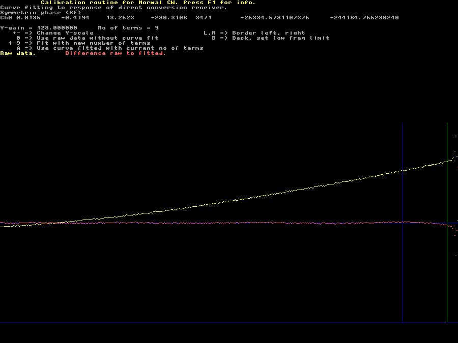
Fig 4. Here the number of terms is 9. Compare with figure 3. | |
|
Even with 9 terms the red line is not zero outside the
excluded region.
The reason is that the symmetric phase curve has a shape that can not be
well fitted to a polynomial.
The errors made by using the polynomial at the right hand side of the
blue line in figure 4 are very small.
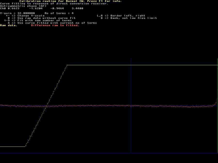
By doing the calibration using a lower repetition frequency for the calibration pulses one can set the excluded frequency range smaller. By calibrating from the blankerinit4.raw file that has a 10 times lower pulse repetition frequency one can set the excluded range to 50 Hz and find that 9 terms is actually enough to describe the phase response of the RF section. The poor fit for the many term polynomials indicates that the procedure is not well written. Maybe something other than a polynomial would fit better - or perhaps the fitting is made over a too wide range. Linrad may improve on this point some day which might make calibration the calibration procedure easier to understand, but probably not affect performance at all. Running the calibration procedure at a very low pulse rate shows another thing that is illustrated by figure 5. | |

Fig 5. Compare with figure 3. | |
|
The second polynomial fit, the antisymmetric phase, shows the phase
response of the audio section.
By using the blankerinit4.raw file which uses a 5 Hz square wave
to give a 10 Hz pulse repetition frequency,
the width of the center discontinuity should be well below 50 Hz
which is where the green line of figure 5 is placed.
It is obvious that there is a phase shift that starts already
around 200 Hz and this is due to the DC blocking high pass
filters in the hardware and in the digital DC restoring
algorithm of the soundcard.
Currently (vers 02-39) Linrad does not allow a fit to this phase shift.
For the WSE units it does not matter,
the phase shift is small over a narrow frequency range only.
With other hardware, particularly if the DC blocking filters are also used to attenuate the mains frequency and its overtones, it might be a good idea to add terms to fit to the phase and amplitude response of the audio section at low frequencies. With the ability of Linrad-02.28 and later to calibrate from files it will be possible to investigate this if someone has such hardware. When blankerinit5.raw is used for calibration, the time window for each pulse is so short that the total number of points in the flat region of the pulse is only about 100 so a pulse is described by an fft in 100 points only. Figure 6 shows one of the center notch screens with a width of 1500 Hz for the excluded points range. The result of the calibration is not quite as good as with a lower pulse repetition frequency. | |

Fig 6. At high pulse repetition rates the transforms become smaller and the center notch wider. At some point the accuracy will suffer. | |