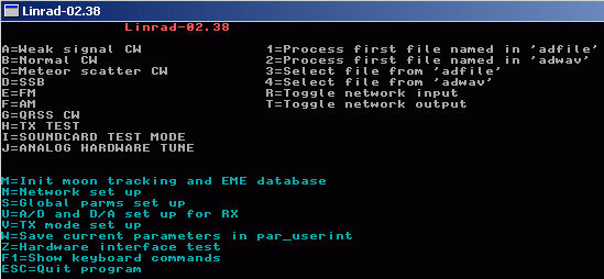
Fig 1. The main menu of Linrad.
About this page.The purpose of this page is to provide some understanding of the calibration procedure used in Linrad. This page demonstrates how to calibrate one particular hardware unit that I was using for EME in about 1995. The file containing calibration pulses can be downloaded and used to produce the calibration files dsp_xxx_corr that would work with this particular hardware.Erase any dsp_xxx_corr file that may be present in your Linrad directory (or create a new Linrad directory without such files.) Download the file containing calibration pulses and go through the calibration procedure to become familiar with it. Finally erase the dsp_xxx_corr files. They are of no use with your own hardware. With the experience you will get it should be easier to perform the calibration on your own hardware. Hardware and raw data.The calibration pulses are contained in http://www.sm5bsz.com/linuxdsp/flat/cal1/blankerinit1.wav (8 155 062 bytes) This file was recorded on a DAT recorder many years ago using the hardware described here Hardware for PC receiver.This hardware was optimised for Soundblaster 16 soundcards with a maximum sampling speed of 44.1 kHz and a 200 MHz Pentium MMX. The DAT recorder was however oversampling at 48 kHz. To do the calibration procedure from the blankerinit1.wav file as described on this page, place the file in a directory /wavlib if you run under Linux or in a directory c:\wavlib if you run under Windows. Then place a file adwav or adwav.txt in the directory from where you launch Linrad. Use one of these files adwav for Linux or adwav.txt for Windows depending on the OS you are using. You also have to create a subdirectory par under wavlib. This is where Linrad will place the parameter files for this recording as specified in the adwav file. Running for the first timeThe linrad main menu, figure 1, gives two options to process a wav file. Press 2 if you actually use the adwav file from this page or press 4 to select one of the lines of the adwav file you are actually using if your adwav file contains several lines. When running for the first time Linrad will prompt for the receive mode to use, figure 2. Select any mode, i.e. SSB.You must then answer Y to the question Repeat recording endlessly because Linrad will read from the file at 48000 samples per second while you set filter parameters and Linrad will hang in the calibration routine if end of file is reached. Answer N to the next question shown in figure 3. | |

Fig 1. The main menu of Linrad. | |
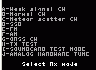
Fig 2. Select the mode for processing a recorded file. | |
|
Fig 3. Answer Y to the first and N to the second question. | |
|
Linrad will remember your choices in the file blnkini_1
under the par subdirectory under wavlib as specified in adwav.
You will then most probably be prompted for the mode parameters.
The parameter files in your Linrad directory (if you have any) do
most probably not match 48 kHz real valued signals.
What parameters you select does not matter much for the calibration,
the Linrad standard parameters should be fine,
but you may also try different bandwidths for the first fft which
could affect the timing but that should not affect the final result.
Other parameters have no influence at all on the calibration.
(But they do affect the receive performance as demonstrated further
down this page.)
When the parameter selection is finished you should see a screen similar to the one shown in figure 4 after moving around the windows, disabling the blanker and adjusting the controls for the timf2 oscilloscope. (Use the F1 help to find out how to do these things.) Figure 4 shows serious processing errors, parameters have to be adjusted, but that can wait until after the calibration is finished. Optimum processing parameters may depend on how the calibration is done. | |
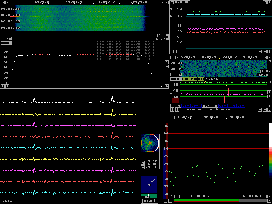
Fig 4. The receive screen of Linrad with default parameters using the file blankerinit1.wav for input. | |
Pulse generator verification.Press X then C and finally A to get to the first screen of the calibration procedure, figure 5. This screen is intended to help setting the amplitude and repetition rate of the pulse generator so it totally useless when calibrating from recorded data which can not be changed. This screen is also intended for verifying that the quality of the pulse generator is good enough and that there is not too much interference. The yellow traces are the two channels in linear amplitude scale while the white trace is summed power in a logarithmic scale. | |
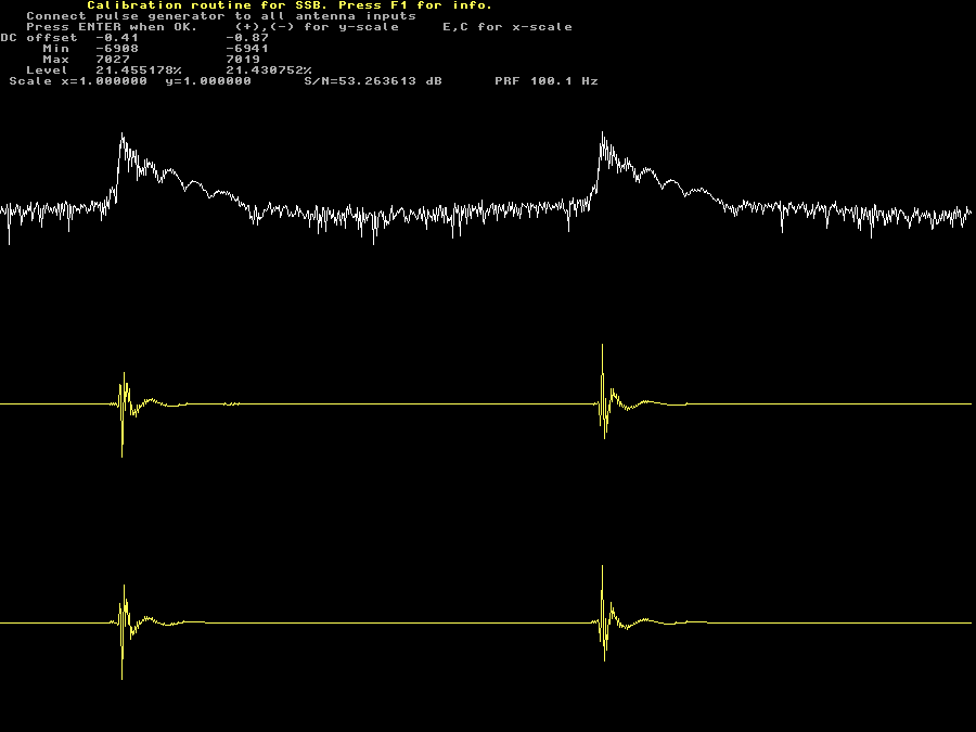
Fig 5. The pulse generator verification screen. | |
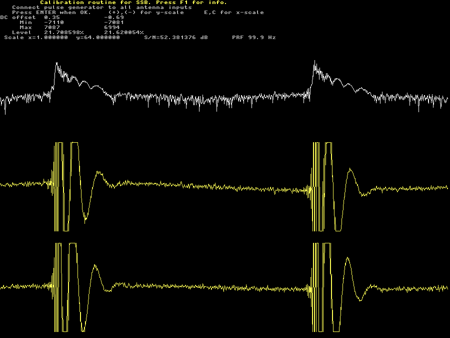
Fig 6. 64 times magnified pulse generator verification screen. | |
Figure 6 shows the same screen as figure 5 after pressing + 6 times.
(It is not the same pulses. The file contains many pulses and the phase differs
from pulse to pulse.)
The vertical gain on the yellow amplitude traces are 64 times larger in
figure 6 as compared to figure 5.
One can see that the pulse amplitude in figure 5 is about 55 pixels
while the noise amplitude in figure 6 is about 5 pixels.
S/N is therefore about 64*55/5 = 704 or 57 dB.
Linrad computes S/N to 53 dB because the DC voltage between the pulses
is not flat and Linrad takes the deviation for noise.
Collect the average pulse shape.By pressing enter on the pulse verification screen you get to the screen where the average pulse shape is collected. See figure 7. | |
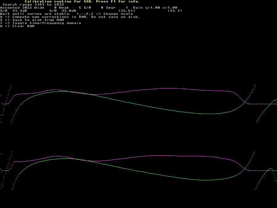
Fig 7. The screen for collecting average pulse shapes. | |
|
In 30 seconds Linrad will collect the average of 3000 pulses
which is more than enough considering the good S/N of the
pulses in the blankerinit1.wav file.
While in the collecting averages screen you may press T to see the individual pulses as they are collected or rejected. With the blankerinit1.wav file the result is as shown in figure 8 on which + is pressed 8 times to magnify the amplitude 8 times. Looking at the pulses on this screen should help to understand the calibration procedure. | |
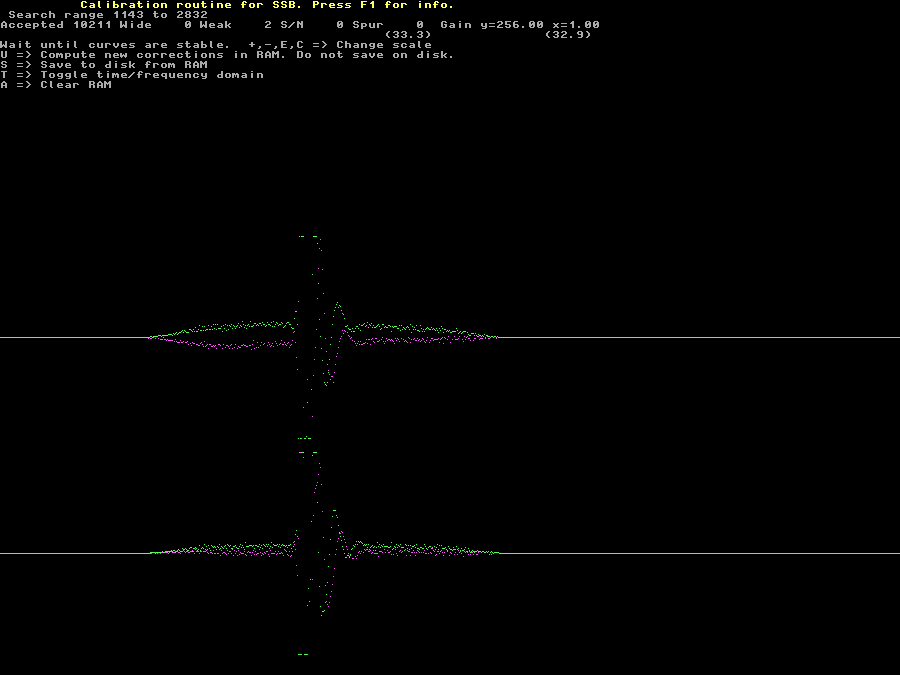
Fig 8. Individual pulses on the screen for collecting average pulse shapes. | |
| The actual pulse showed in figure 8 lasts for about 65 pixels only. The DC voltage around the pulse is undetermined however and that presents a difficulty. The origin of a non-flat background for the pulses is partly the mains frequency and its overtones, partly low frequency noise of unknown origin. Figure 9 shows the blankerinit1.wav file as seen with a wave-file editor (Creative Wave Studio.) The signal is amplified by a factor of 256 just as the signal in figure 8. | |
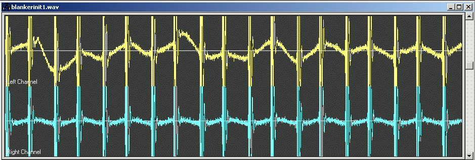
Fig 9. The pulses in blankerinit1.wav as seen with a wave-file editor. Tha amplitude is magnified by 256 to make the pulses comparable to the ones in figure 8. | |
|
Figure 8 is in complex format (I and Q) at 24 kHz sampling rate while
figure 9 is in real format at 48 kHz.
This does not change the general picture however.
The big difference between figures 8 and 9 is that a window
function is applied in Linrad to force the background to zero
at both ends of the sequence.
This window is a cosine squared function over 25% of the time
at both ends with a flat region in between for the pulse.
It should be pretty obvious that correct calibration
can be obtained only if the entire pulse is within the
flat part of the window function.
For this reason the pulse repetition frequency has to be low
enough to make the pulse and all its oscillations down
to the noise floor last no more than 25 % of the time
between two consecutive pulses.
Actually the requirement is a little less stringent because
the window functions overlap to some extent.
Without the cosine squared that modulates the DC component with low frequencies so it goes to zero at both ends of the sequence there would have been a discontinuity in the time function that would have added contributions on all frequencies. The fourier transform actually computes the spectrum of an infinite sequence where the same data points repeat again and again and if the last point in the sequence does not fit to the first one, the misfit will generate overtones. The cosine squared modulation of the DC component is well taken care of by the pulse averaging routine, it is present only in a few points of the transform. With a rectangular window to pick out a pulse and its surroundings, the transients cause signals in all frequency bins and makes the computation of the average more difficult. The problem is that one can not average the pulses directly because they would then average out to zero because their phase is random. The averaging is done in the frequency domain where amplitudes and phases are averaged separately (actually the second derivative of the phases.) A phase is undetermined in the number of turns. When an error of 2*PI (360 degrees) is made just once for just one pulse, the entire result becomes incorrect. The risk is greatly reduced by not having the large random contributions from a wideband pulse present in the transform. With a pulse repetition rate of 100 Hz like in the blankerinit1.wav file, the total time spanned by the window function is only about 5 milliseconds. This means that the lowest frequency that can be represented is 200 Hz when the pulse is transformed to the frequency domain with an FFT. Lower frequencies will show up in the DC component which will vary from transform to transform and average out to zero provided that the phase of the pulse is random with respect to the mains frequency. The pulse generator used to generate the blankerinit1.wav file was a digital IC converting the 50Hz mains frequency to a square wave. The square wave was filtered through a 144 MHz band pass filter followed by a class C amplifier. The phase jitter on the 50 Hz square wave was large enough to make the phase of the pulses reasonably random with respect to each other. As can be seen in figure 7, the first two pixels at the left side of the spectrum has large amplitudes. Much more so in the upper channel than in the lower. This is an artifact caused by the low frequency components that do not average out completely. These points are obviously outside the true passband so they present no problem. Set the desired filter response.By pressing U on the collect average pulses screen you reach the screen for setting the desired filter response, figure 10. | |
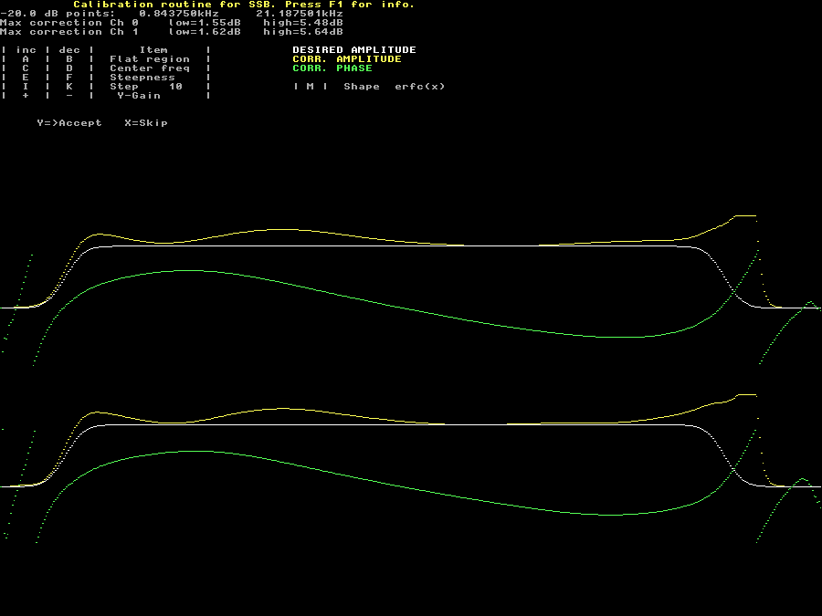
Fig 10. Set the shape of the total filter response in Linrad on this screen. | |
|
The white curve is the desired filter response.
Obviously it is perfectly flat over a wide range and it is
identical in both channels.
Linrad uses the information contained in the average pulse response
to construct a digital filter that is applied to the input signal
before its spectrum is displayed on screen for the total filter
response to become as desired.
The gain of this digital filter is the yellow curve and they are slightly
different between the two channels.
The green curve is the phase response of the digital filter Linrad will
add.
This phase function will make the phase response of the entire system
perfectly linear.
What filter response to select may depend on the circumstances. With a very wide flat region Linrad has to apply very high gain at the spectrum edges and that may degrade the system noise figure towards the spectrum ends. On quiet microwave bands one can compensate by setting the front end gain high enough to overcome a degraded noise floor, but more gain means lower system IP3 in the wide center region where the noise figure will not benefit at all from more gain. A very wide flat region gives a peak with strong curvature in the desired amplitude. This is OK only as long as the thermal stability is good enough for the hardware filter chain to match this peak over the temperature range of interest. The steepness of the filter edges, the Q of the entire filter chain, will affect the length in time for the oscillations that surround each interference pulse. On crowded HF bands where the filter has many notches to remove strong signals it might be clever to use a low Q on the total filter chain. Just press Y on this screen to accept the default suggestion for the blankerinit1.wav file. Linrad will then store the digital filter and show the collect averages screen again. Now it looks like figure 11. If it looks good, press S on this screen to save the new filter on the hard disk. | |
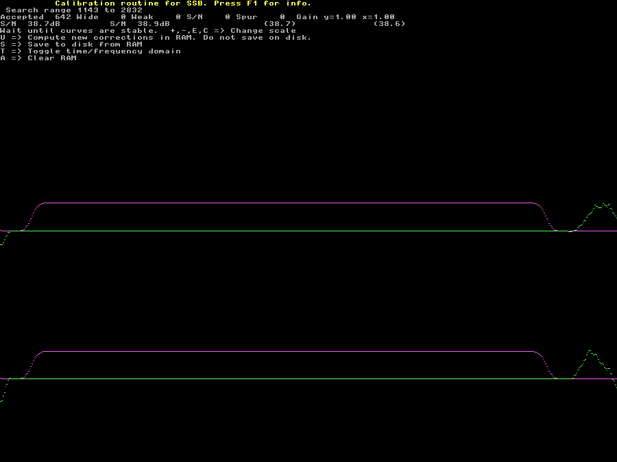
Fig 11. With the new filter in RAM the average collect shows the new filter response for the entire system. | |
Using the new filter function.Linrad has a routine for reducing the number of points in a calibration function. It is Refine amplitude and phase correction This routine will make the digital filter smoother and also reduce the size of the calibration function. With a very good S/N for the pulses and with a high pulse repetition frequency, there is no need to use this function. It will actually degrade blanker performance slightly.Pressing X on figure 11, then again on the next screen to not do "Refine" will bring you to the normal receive screen which will look like figure 12. | |
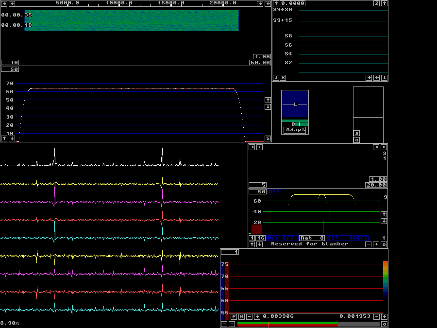
Fig 12. When the calibration is complete, but with the Linrad default processing parameters the receive screen looks like this. Compare this to figure 4 above. | |
|
The default parameters of Linrad cause a serious error that
is visible in figure 12.
The main spectrum has a very large number of red points at
frequencies where Linrad believes there is a strong narrowband
signal.
These red points move around rapidly at random and generate
needless noise as the associated notches are switched on and off.
There are several ways to get around this problem,
one can reduce "First FFT amplitude", "Sellim maxlevel"
or "Second FFT bandwidth factor" or any combination of them.
Which way to go depends on the circumstances.
For details, look here
set digital signal levels correctly.
In figure 13, the "First FFT amplitude" is reduced by 10 dB from 1000 to 316. The "First backward FFT att. N" is also increased from 4 to 5. | |
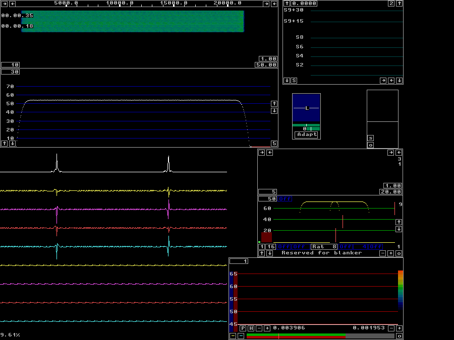
Fig 13.Calibrated, without blanker, but with parameters that avoid saturation. | |
|
Figure 14 shows what happens when the noise blanker is enabled.
The S-meter graph in the upper right corner shows how the
adaptive polarisation routine slowly adapts to the appearent
polarisation of the incoming noise.
It starts assuming the polarisation is horizontal, but ends up
with a polarisation near 45 degrees reflecting that the pulses
are the same in both channels.
The green and magenta curves show peak power while the blue and
red show RMS power.
Both with in the bandwidth of about 400 Hz specified by the yellow
curve in the baseband graph.
When the smart blanker is switched on, the RMS noise drops from
S9+10dB to just below S4, an improvement of little more than 40 dB.
When the dumb blanker is also switched on,
there is no difference near the passband center,
but the region within which the interference is completely removed
becomes much wider.
Use the blankerinit1.wav file to find out what happens with the pulse shapes when different filter shapes are selected. What it means to real life performance of the blanker is less obvious since it depencs on whether the interference one wants to fight really is wideband enough to be shaped by the Linrad system and to which extent strong signals force Linrad to apply many notches. The amplitude of each interference pulse and their repetition frequency will also have some influence. At the present time I do not know how to operate the Linrad blankers well onder different circumstances. That is why Linrad-02.39 and later allow calibration from saved files. This will make it possible to collect a library of interference situations on different bands with associated files containing calibration pulses for the same hardware. | |
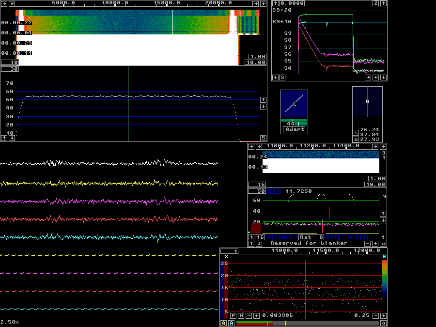
Fig 14.Calibrated, blankers switched on, one after the other. See text. | |