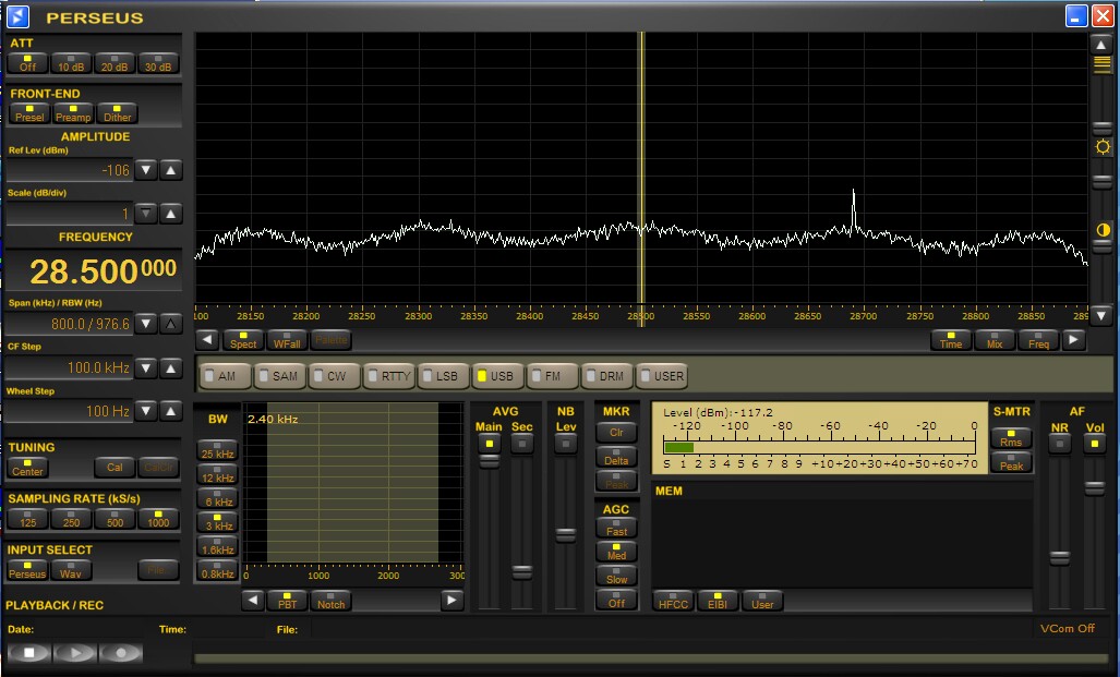
Fig 1. The Perseus spectrum screen with the reference signal at 28.69 MHz.
|
When displaying 1 MHz with about 1000 pixels on a screen, the
bandwidth for each pixel is 1kHz.
The FFT with a corresponding bandwidth would produce a new
line in the waterfall about 1000 times per second.
Averaging has to be used to present the waterfall graph at a
suitable speed.
The sensitivity depends on the amount of averaging and on how
the averages are computed.
Linrad is designed for flexibility and optimum performance which makes it a bit difficult to learn to use in full. The Perseus and Winrad software on the other hand are designed for user-friendliness. In order to demonstrate the sensitivities of the waterfall graphs of the different software, a Compaq 6510b laptop was connected to the Perseus hardware which in turn was connected to a signal source with four signals generated by four HP8657A signal generators. The generators were connected to a four way splitter feeding a wideband RF amplifier which served the purpose to lift the noise floor slightly (about 7 dB.) One signal was set at a reference level that allowed detection on the main spectrum of Winrad and Perseus. The other generators were set 10, 20 and 25 dB below this level. Figures 1 and 2 shows the screen of the Perseus software with spectrum respectively waterfall displays. |
|
Fig 1. The Perseus spectrum screen with the reference signal at 28.69 MHz. |
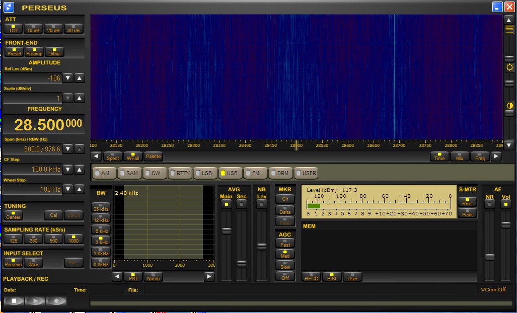
Fig 2. The Perseus waterfall screen with the reference signal at 28.69 MHz. |
|
The reference signal has (S+N)/N = 2dB in the Perseus
main spectrum and it is well visible in the waterfall while
the 10 dB weaker signal at 28.31 MHz is not quite visible in the
waterfall although it seems to be at (S+N)/N = 0.3 dB in the main
spectrum.
Figure 3 shows the same signals with Winrad. The averaging is similar to that of the Perseus software. The reference signal has (S+N)/N = 1dB in the main spectrum and it is well wisible in the wide waterfall. |
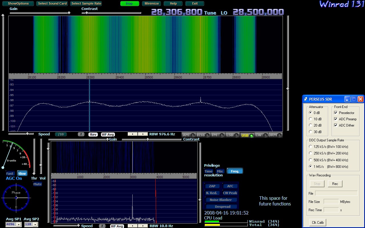
Fig 3. The Winrad screen with the reference signal at 28.69 MHz. |
|
A comparison between the Perseus software and Winrad shows that both
of them have similar sensitivity for weak signals in the wide waterfall
graph as well as in the wide spectrum display.
Linrad is dramatically different.
Figure 4 shows the Linrad screen with the same input as for all other
images on this page.
|
Fig 4. The uncalibrated Linrad screen with the reference signal at 28.69 MHz. The 10 dB weaker signal at 28.31 MHz is well visible in the main spectrum. The signal 25 dB below the reference signal is marginally visible in the 1 MHz wide spectrum, but it is well visible at 28.699867 MHz in the baseband spectrum and waterfall. |
|
The filters used by the FPGA in the Perseus hardware has about 1 dB
ripple, something that can be seen to some extent also on the
Winrad waterfall.
By running the standard calibration procedure of Linrad it is possible
to correct for this.
Figure 5 shows the same three signals when Linrad is calibrated.
|
Fig 5. The calibrated Linrad screen with the reference signal at 28.69 MHz. The 10 dB weaker signal at 28.31 MHz is well visible in the main spectrum. The weaker signals are only visible in the waterfall. |
The signal in the baseband waterfall is about 8 dB above the noise
in a bandwidth of 0.5 Hz.
From this we can conclude that the signal levels are:
  Freq      Level
 (MHz)     (dB/Hz)
28.70         5
28.48        10
28.31        20
28.69        30
The source of the signal at 28.688 MHz is unknown while the signal at 28.500 MHz is the zero spur which is generated by rounding errors. It should be clear from the images above that Linrad is about 15 dB more sensitive than conventional software when it comes to chasing weak signals in a wide waterfall. The reason is that Linrad computes averages point by point in a large FFT. In figures 4 and 5 the FFT size is 262144 with an associated bin bandwidth of about 10 Hz and about 250 FFT bins for each pixel. The display shows the strongest average out of about 250 ones for each pixel. Since each FFT bin is an average of 200 transforms, the noise floor becomes very flat and therefore a high gain can be used for the colour scale. The high resolution graph shows the average over 200 transforms with one pixel per bin. The entire window is 510 FFT bins so it corresponds to only 2 pixels in the main spectrum. It is obvious that the 28.70 MHz signal is about 1 dB stronger than the strongest bin in surrounding regions regions of 250 points. That is why it is visible in the waterfall. The 28.70 MHz signal which is at 5dB/Hz should be at -5dB in 10 Hz bandwidth. This converts to a factor of 0.31 in linear power scale. We should therefore expect (S+N)/N to be 1.31 in linear power scale which converts to 1.2 dB in good agreement with what can be seen in figure 4. The strongest bin has three times more noise than signal. In the averaged spectrum, the noise fluctuates within a band that is about 1 dB wide, so sometimes the noise plus signal is not stronger than the strongest bin in surrounding regions, sometimes it is more than 2 dB stronger. The time to collect 262144 samples is 0.26 seconds but the transforms are windowed and overlapping by a factor of two so the average over 200 transforms spans a time of 26 seconds. The time constant of Winrad is -6 dB for 180 seconds with the recommended settings for best sensitivity. This means that it takes about half an hour for a strong signal to disappear from the colour graph. I do not think it is corret to call this graph a waterfall because it is just an array of vertical lines in different colours. Considering the time constant, the lines should be drawn at a rate of about one line per minute to allow the user to see how (the averaged) signal changes by time. The Perseus software allows a slow waterfall, but not slow enough to fit the maximum averaging allowed. At the minimum speed, about one line per second, a reasonable maximum time constant is like in figure 2 where noise peaks last for about one minute. The sensitivity of Linrad demonstrated above is for signal bandwidths up to 10 Hz. The signal has to last for about one minute and it must not drift by more than about 10 Hz per minute to allow full sensitivity. Larger transforms allow higher sensitivity but put stronger requirements on the stability of the signals. Conventional waterfall graphs that would have a resolution of about 1 kHz when averaging over time and frequency to sum up the energy within the range represented by one pixel have a S/N penalty of 20 dB compared to Linrad due to the bandwidth difference when Linrad is set as shown on this page. Smaller transforms (or equivalently averaging over frequencies) restores a little of this loss, but incoherent averaging is inefficient at S/N ratios well below unity. To SM 5 BSZ Main Page |