This article has been published in DUBUS 4/2003 and it is protected by copyright. Any reproduction, publishing in the Internet or commercial use only with the written permission from the publisher Verlag Joachim Kraft DUBUS Web page
This article has also been published in DUBUS TECHNIK VI 48 - 378 as well as in CQ VHF in two parts, Fall 2004 and Winter 2005.
Receiver
Dynamic Range
Leif Asbrink, SM5BSZ
http://www.sm5bsz.com/index.htm
Receiver dynamic range is the ability of a receiver to receive a weak signal without loss of readability while a strong signal is present. The general concept is very easy to understand but sometimes the published measurements are based on non-valid assumptions. They may actually be measuring something else, which means that published dynamic range data can not be used as the basis for selecting the better of two transceivers. By use of a measurement method that actually mimics the critical situation, it is easy to get reproducible and well defined receiver dynamic range data.
This article will focus mainly on VHF receivers, but most of the comments are relevant at all frequencies.
1. INTRODUCTION
The traditional figures of merit for the dynamic range of a receiver are the third order intermodulation intercept point IP3 and the blocking dynamic range BDR. Actually there are many different receiver overload effects, and each one defines the upper end of a separate dynamic range; but the receiver’s responses to third order intermodulation and blocking are generally assumed to be a good indication of its overall strong-signal handling capabilities.Different authors define and measure BDR completely differently. But even though the definition of IP3 is always the same, the measurement procedures defined to measure IP3 may differ – and some measurements do not actually measure
Let us start from the beginning with these fundamental definitions:
| 0) |
Noise floor power density(NPD).
Receiver noise power level in a 1Hz bandwidth (W/Hz or dBm/Hz), referred
to the receiver input.
This is the lower end of all the dynamic ranges defined below.
On the air, noise floor power density is a property of the receiving system, because in addition to the receiver noise temperature TRX it must include the effective noise temperature of the antenna system: NPD = k(TRX + TANT) For dynamic range measurements, the receiver input is always connected to some kind of resistor (e.g. the output attenuator of a signal generator) which generates thermal noise. If this resistor is assumed to be at 290K, it can be shown that: NPD = –174 + NFRX dBm/Hz (2) where NFRX is the receiver noise figure (dB). Equation (2) is actually one way of formulating the definition of the noise figure. |
| 1) | One-signal dynamic range. Max undistorted level of a single desired signal in the receiver passband. Measured in dB above the noise floor power density. |
| 2) | Two-signal dynamic range Max level of a single undesired signal that will degrade the S/N of a very weak desired signal by 3dB or less. Measured in dB above the noise floor power density. The two signal dynamic range is a function of the frequency separation. |
| 3) | Three signal dynamic range Max level of two equally strong undesired signals that will not produce intermodulation products above the noise floor. Measured in dB above the noise floor power density. |
Traditional definitions measure dynamic ranges in a specified bandwidth. Different product reviewers use actual CW or SSB bandwidth of the receiver, or some may recalculate the data to a standard 500Hz or 2.5kHz bandwidth. Defining the dynamic range in relation to the power density of the noise floor (dBm/Hz instead of just dBm) normalizes all measurements to a 1Hz bandwidth. This avoids ambiguity and is also very convenient for the measurement methods described below, where the output of a receiver is measured with an audio spectrum analyzer.
2. THE ONE-SIGNAL DYNAMIC RANGE
When you tune to a really strong SSB signal, the audio output may become severely distorted. This is not much of a problem for amateur SSB, but it is important for some data modes and may be essential in other services. The in-channel distortion caused by receiver overload can be avoided by use of better AGC circuits, ultimately an AGC-controlled RF attenuator at the antenna input as described by Ulrich Rohde in ref. [1]. There is no limit for how high one can make the one-signal dynamic range this way, but when AGC is used the signal/noise (S/N) ratio does not continue to improve. Since the one-signal dynamic range is not relevant to the main subject of this article, I see no reason in going deeper into measurement procedures. The one-signal dynamic range is closely related to blocking, as explained later.3. THE TWO-SIGNAL DYNAMIC RANGE
This is the most important quality of a VHF receiver. In principle, the measurement procedure is very simple: Set the signal level of a first signal generator to a suitable low level. Monitor the S/N of this signal with an audio spectrum analyzer at the audio output. Then increase the level of a second signal generator (PGEN) until S/N is degraded by 3dB. The level of the second generator in relation to the noise floor power density is the two-signal dynamic range.DR2 (dBHz) = PGEN(dBm) – NPD(dBm/Hz) (3)
(The units of DR2 are dB. The abbreviation dBHz should be read as “dB, referred to a 1Hz bandwidth”.)
The degradation of the S/N can occur by several different mechanisms that either reduce the signal or increase the noise level. These mechanisms are discussed further at the end of this section, but the main two are identified here. Reduction of the signal level is called blocking, and is discussed below. A noise-free strong signal can cause an increase in the noise level due to reciprocal mixing between that signal and the noise sidebands of the receiver’s local oscillator. The two signal dynamic range measurement, as defined here, does not question which of these two effects is happening, or what the causes are - it simply measures the practical total effect upon S/N. That is all a receiver reviewer needs to measure, because it shows readers what will happen on the air. Only the receiver designer needs to measure blocking and reciprocal mixing separately, because the ways to improve them lie in different parts of the receiver.
The two signal dynamic range varies with the frequency offset between the wanted and unwanted signal, in a way that depends on the receiver architecture. When the mechanism is reciprocal mixing, DR2 follows the spectrum of the sideband noise on the local oscillator(s) but when the mechanism is blocking it depends on which stage of the receiver is the one that overloads, and how much effective selectivity there is before that stage when the mechanism is blocking.
The practical problem with DR2 measurement is that the strong signal generator must not produce significant sideband noise at the frequency to which the receiver is tuned. This is where a crystal filter is needed. On HF bands it is possible to use the steep edge of a crystal bandpass filter to remove the sideband noise from the strong signal but on VHF this is not possible; a crystal notch filter must be used instead (see later). At VHF, normal crystals do not like the power levels needed to test good receivers. It is of course possible to make very low noise crystal oscillators for this test, but it is not so easy to be sure the test oscillator really is as good as one thinks.
The definition of DR2 above is closely related to the conventional definition of blocking dynamic range, BDR [3-8]. The amount of degradation associated with the DR2 value as I have defined it here is 3dB, rather than 1dB, which is often used in other definitions. The reason to use 3dB in the definition is twofold. First, the measurement is faster. This is important because the whole measurement must be repeated at several frequency offsets to see the complete picture. When the S/N degradation mechanism is reciprocal mixing and one wants to find the level of the strong signal within 1dB, one has to measure the noise floor very accurately if one wants to determine the level of the strong signal within +/- 1dB - as can be seen from Table 1. The 1dB degradation calls for a noise level measurement within +/– 0.1dB, which in narrow bandwidths takes a lot of time to achieve statistical accuracy. For the 3dB degradation, +/- 0.25dB is sufficient accuracy for each noise level, saving a factor of 6 in time.
|
Added noise signal relative to main signal (dB) |
Signal level |
|
-30 |
0.00 |
|
-20 |
0.04 |
|
-15 |
0.13 |
|
-10 |
0.41 |
|
-9 |
0.51 |
|
-8 |
0.64 |
|
-7 |
0.79 |
|
-6 |
0.97 |
|
-5 |
1.19 |
|
-4 |
1.46 |
|
-3 |
1.76 |
|
-2 |
2.12 |
|
-1 |
2.54 |
|
0 |
3.01 |
|
+1 |
3.54 |
Table 1. Adding a second noise source increases the noise level like this. For example, if both noise levels are equal (0dB), the sum is 3.01dB above a single signal and the sensitivity is about +/-0.5dB for a +/-1dB change of the added noise. If the added noise is 6dB below the original noise, the sum is 0.97dB above the original noise but the sensitivity is only about +/-0.2dB for a +/-1dB change of the added signal.
The BDR (blocking dynamic range) values measured by ARRL lab and published in QST show when a receiver is blocked, and these BDR values can be taken to be one-signal dynamic range values if the measurement is not “noise limited”. (Note that ARRL have their own definition for BDR through the ‘ARRL Standard’ BDR Test Conditions in ref. [2].) For example, the BDR value for the FT1000D published by ARRL lab is “larger than 154dB”; that refers to a bandwidth of 500Hz, so by the definitions above the one-signal dynamic range of the FT1000D is more than 181dBHz.
The second reason for using 3dB degradation rather than 1dB when measuring DR2 is that for a receiver in which performance is limited by reciprocal mixing only, the numerical values become equal to the oscillator phase noise (dBc/Hz). Comparing the receiver DR2 to the transmitter sideband noise may also show if there is a further problem caused by noise modulation in the transmitter amplifier stages (a common problem).
As noted above, the definition of DR2 does not discriminate between the many different mechanisms that may be the reason for loss of S/N for the desired signal. This list of possible mechanisms is not complete, it just contains phenomena I have encountered in real life:
| 1) | Blocking – the sensitivity of a saturated receiver is degraded. |
| 2) | Reciprocal mixing – due to phase noise from the local oscillator. |
| 3) | Amplitude modulation in RF amplifiers or LO buffer amplifiers. |
| 4) | Phase noise (time jitter) in CMOS switched mixers. |
| 5) | Phase noise in (time jitter) in frequency dividers. |
| 6) | Noise bursts caused by movement of small particles inside ceramic capacitors. |
The list should also include wideband interference caused by strong signals. On top of that there are the discrete spurious responses. At some particular frequency separations there are false responses for the strong signal, and such spurs degrade DR2 at those frequencies. As well as giving the wideband performance, preferably as a graph, the complete DR2 performance should include a list of spurs, but presenting such a list is not as simple as it first seems. First order spurs like the mirror image frequency could be tabulated formally as DR2 numbers for specific frequencies, because the DR2 value equals the spur suppression in dB. However, receivers also have higher order spurs, things like (8*LO-5*RF) which may appear at very high RF signal levels whenever the result becomes equal to the IF frequency. Applying the DR2 definition directly is impossible for these higher order spurs, because the result will depend on what signal level one has chosen for the weak signal. One way of describing higher order spurs is as a list stating: the frequency; what the level of the spur is for an input signal close to the wideband DR2 level; and the order of the spur, which tells you by how many dB it decreases when the input level is reduced by 1dB.
4. THREE-SIGNAL DYNAMIC RANGE
The measurement is conceptually simple: Set the signal level of a first signal generator to a suitable low level. Then increase the levels of a second and a third signal generator until the level of the third order intermodulation product equals the level of the weak signal as measured with an audio spectrum analyzer at the audio output. The second and third signal generator should have equal amplitudes and their frequencies have to be set for the third order intermodulation product to be within the receiver passband.When measured this way, the third order intermodulation product accurately follows the theoretical third order law, because the first signal is used as a pilot tone that makes the measurement unaffected by AGC circuits after the IF filter. If the receiver uses dual-loop AGC [4], the third order law will not hold at signal levels high enough to make the AGC reduce the RF gain.
With PW for the power of the first generator in dBm and PS for generators 2 and 3, the third order law is like this:
3PS (dBm) = PW (dBm) + 2k (dBm) (4)
where k is a constant, identified below.
If the power level of the generator 1 (PW) is set to equal the NFPD, and the output powers of generators 2 and 3 (PS) are increased together until the third order intermodulation product appears at the same level as PW, then the third order dynamic range DR3 is simply the difference in dB between PS and PW. The formula becomes:
DR3 (dBHz) = PS (dBm) – NPD (dBm/Hz) -
{ PW (dBm) – NPD (dBm/Hz)}/3 (5)
The constant k in equation (4) is in fact the third order intercept point IP3 (dBm). This is the point where PS and PW would become equal if the third order law continued to be valid at such high levels. It follows that:
IP3 (dBm) = PS (dBm) + {PS (dBm) – PW (dBm)}/2 (6)
As a figure of merit for a receiver, IP3 is meaningless unless it is specified together with the associated noise floor. Just by adding a 10 dB attenuator, one would improve IP3 by 10 dB but the distance between IP3 and the noise floor would not improve since the noise floor would be raised by 10 dB also. One can specify IP3 in dB above the noise floor in 1 Hz like this:
IP3 (dBHz) = PS (dBm) + {PS (dBm) – PW (dBm)}/2
– NPD (dBm/Hz) (7)
The IP3 number that comes out is typically about 10dB larger than the DR2 value in the cases where DR2 is determined by blocking. This is relevant to the designer who wants to separate blocking from reciprocal mixing. IP3(dBHz) and DR3 convey the same information and for a receiver comparison one can use either one. They are related by:
DR3 (dBHz) = 2/3 * IP3 (dBHz) (8)
In a 500 Hz bandwidth the noise floor is 27dB higher, which gives:
DR3 (500Hz) = DR3 (dBHz) – 18 nbsp; (9)
The complete intermodulation dynamic range characteristics of a receiver should also include information about intermodulation of second order, and also of fourth and higher orders. Second order intermodulation can be very important for HF receivers, where a broadband front-end can allow second order intermodulation between say two 7MHz signals with the product causing interference at 14MHz, but it is normally of little interest on the VHF bands where we routinely use narrow filters at the RF frequency. Fourth and higher orders occur only near saturation when lower order IMD is already very strong, so these are of very little practical interest.
Note that intermodulation performance is a function of frequency separation of the two unwanted signals from the wanted frequency. This is for essentially the same reasons as blocking, namely the amount of effective selectivity ahead of the stage(s) that suffer intermodulation. It also means that a full intermodulation report will be quite an extensive table.
5. THE MEANING OF IP3
The third order intercept point, IP3, although a number that is obtained
from an extrapolation, has a real physical meaning and it is well defined.
The fact that different standardized procedures give different results
may be because not all of these procedures measure IP3 correctly.
They may be based on incorrect assumptions or some theoretical mistake.
Another thing is that IP3 and the theory behind it is not applicable on
all receivers.
The most obvious case is a DSP radio containing an A/D converter in the
signal path.
However, analog receivers may also have side circuits such as noise blankers
that contain amplifiers that produce intermodulation at signal levels
where the main signal path is very linear.
Such intermodulation may leak into the main signal path due to inadequate
screening or buffering, causing irregular behaviour at low signal levels.
A single stage that causes intermodulation can be described by a transfer function that is very close to a straight line for voltages well below saturation. If the input is denoted X(t), a voltage that varies with time, the output Y(t+d) can be described with a power-series expansion in amplitudes only:
Y(t+d) = k1X(t) + k2{X(t)}2 + k3{X(t)}3 + … (10)
where k1, k2, k3 etc. are constant coefficients; and d is the time delay between input and output (not important here).
Such a description is valid if the input signal is small. At larger signal levels, there will also be a phase shift because semiconductors contain a capacitance that varies with the voltage in a non-linear fashion. Any reasonable analog circuitry (mixers, amplifiers, iron cores, whatever) will have k1 > k2 > k3 > … so if the signal levels are really low, the transfer function is well described by the first ‘linear’ term only. By making
X(t)=A* {sin( 2* p * f1 ) + sin( 2 * p * f2 ) } one can easily find what the output signal Y(t+d) becomes. Third order intermodulation is due to k3, k5, k7… and k3 alone is responsible for the third order intermodulation at very low levels. Cascading multiple stages will not change this analysis; the complete cascade of stages will still be characterized by equation (10), but with a new set of coefficients that can be computed from the individual stage coefficients.
IP3, the number we use to express k3 of the transfer function, should have an exact relation to DR3, which is another number we may use to express the same thing. If you find (for example in some QST reviews) that measured IP3 values do not have the correct relation to measured DR3 values, this may indicate a measurement mistake or that the tested receiver has a leakage of intermodulation from some saturated stage that is not part of the signal chain. The ARRL lab measurements of TS-690S [9] show an extreme example, in which the third order intermodulation falls off by only 0.5 dB for an 1 dB reduction of the input level rather than the expected 3 dB. I have looked carefully at a TS-450S which was reported in [9] to have the same behaviour as the TS-690S, but found no sign of that peculiar behaviour. The serial number was much higher and maybe the signal leakage problem had been cured.
IP3 or DR3 are both good figures of merit to describe the analog front-end of a receiver because they are both related to the fundamental transfer equation (10). However, A/D converters used in digital radios are not well described by (10). If multiple strong signals are allowed to enter the A/D converter, the relevant figure of merit is the A/D saturation limit. Below this limit, A/D converters are typically very linear – they produce practically no IM3 all the way up to the saturation limit where they fail completely. A digital receiver will have IP3 and DR3 values that look very good, but in real life they can not be compared to “good old analog” receivers that will continue to function with input voltages high above the range indicated by DR3. For example, an analog receiver that is subjected to 10 signals at the DR3 level will produce IM3 for all combinations of these signals, but these spurious responses will be near the noise floor. A digital receiver will see the 10 signals sometimes add in amplitude to give a peak level that is 20 dB higher, so it may become heavily saturated and useless. At the present state of the art, digital receivers need roofing filters to limit the number of signals entering the A/D converter, but inside the roofing filter bandwidth they remain vulnerable to saturation effects when the band is crowded with very strong signals. Test procedures must take realistic account of this.
A receiver that has a signal leakage at low input levels is not well characterized by an IP3 number. There is no point at and below which the third order intermodulation follows a third-order law. IP3 and DR2 should be presented only if the measurements show that they are valid figures of merit and any observed deviations occur at levels low enough to be insignificant; otherwise the entire curve of intermodulation versus input signal levels should be presented as in [9]. An EME operator looking for signals 20 dB below the SSB bandwidth noise floor might find the TS-690S receiver with the performance reported in [9] completely useless, while other operators not looking for signals below the noise floor might find the leakage insignificant. In real usage on the air, the noise floor is typically 10 to 20 dB higher than during the IM3 measurement, due to noise from the antenna on HF or due to the noise from the tower mounted preamplifier for in weak-signal VHF/UHF usage.
There is a detailed analysis and some accurate measurements at http://antennspecialisten.se/~sm5bsz/dynrange/intermod.htm. This Internet site illustrates the validity and limitations of IP3 and DR3 for characterization of receiver intermodulation.
6. PRACTICAL MEASUREMENT OF NOISE FLOOR
First of all the noise floor has to be established. Methods that use a signal generator and an RMS voltmeter and rely on the known bandwidth of the receiver under test have accuracy problems because the audio frequency response is often not very flat – for example, Fig. 1 shows the frequency response of an IC-706MKIIG.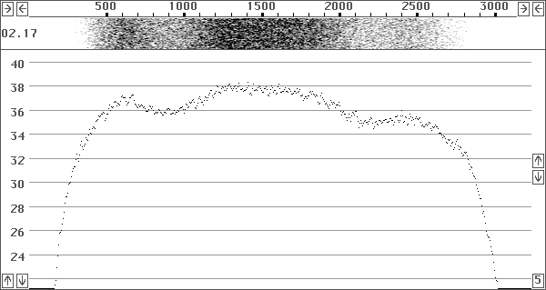
Fig. 1 Frequency response of an IC-706MKIIG. The passband ripple is in the order of +/- 2dB and would be invisible at a “normal” y scale.
A typical (old) procedure would be to use a signal generator and a RMS voltmeter to locate the 6dB points which would be found at about 300Hz and 2800 Hz. One would then place the signal generator at the frequency of maximum and determine at what signal level the reading of the voltmeter has increased by 3dB. This is the point where the signal power equals the noise power, so one would then say that the noise power in 2500 Hz bandwidth equals the power level of the signal generator. The error in taking the 6dB bandwidth rather than the true noise bandwidth (equivalent ‘rectangular’ bandwidth giving the same noise power) will of course depend on the details of the frequency response. For the IC-706MKIIG in Fig.1 the actual noise bandwidth is only 1.6 kHz, so the error is 1.9 dB. All uncertainties add together, so by measuring the noise floor properly we can improve the accuracy of dynamic range measurements by several dB. Using a RMS voltmeter at the output may introduce errors if the AGC is not completely disabled. With a standard multimeter that is not a true RMS voltmeter other uncertainties are added as well.
To measure the sensitivity accurately, an audio spectrum analyzer should be used. These days such instruments are readily available in the form of computer programs for a standard PC computer. There are many alternatives but (since I wrote it myself) I prefer Linrad, which is free Linux software and can be downloaded from http://antennspecialisten.se/~sm5bsz/linuxdsp/linrad.htm
Besides the audio spectrum analyzer, a power reference is needed. It may be a calibrated noise source with a known noise temperature, but it may equally well be a signal generator with a well-known output level near the noise floor.
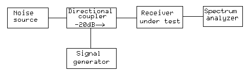
Fig. 2. Setup for NF measurement on a receiver.
The noise source can be switched between two known noise temperatures, usually called ‘hot’ and ‘cold’. If you have access to an old vacuum tube (diode) noise source, the hot noise temperature is known from the anode current by theory. Such noise sources are typically supplied with a plate current meter that is calibrated directly in noise figure and one is supposed to adjust the plate current for the noise level in the receiver to increase by 3dB when the current is switched on. The noise source may also be a semiconductor diode which presumably is calibrated so you know what the ‘hot’ noise temperature is when you give it the prescribed current. Without any current the noise source will have a ‘cold’ noise temperature that equals the room temperature or a little higher, the temperature of the resistor inside the noise source may be a little above room temperature. Noise figures are specified for a standardized temperature of 290K. If you make the measurement with the noise source at a different temperature there will be an error that you should correct if you look for an accurate noise figure.
When the current is switched on in the noise source, there is a side effect besides the increased noise temperature. The impedance will change slightly. In case the gain of the receiver under test is very sensitive to the source impedance, the noise floor will change because of the changed gain also and not only because of the changed noise temperature of the noise source. For the purpose of evaluating dynamic range, a modest accuracy of the NF is sufficient, but for measurements of low noise figures the accuracy has to be much higher. Rainer Bertelsmeier, DJ9BV, has written in detail about these problems [10]. One typically uses an attenuator to reduce this effect because it makes the impedance change smaller, but the noise source should preferably be calibrated with the attenuator permanently in place. With the setup of Fig.2, the purpose of the signal generator and the directional coupler is to supply a pilot signal with constant amplitude. By monitoring it on the audio spectrum analyzer one can compensate for modest changes of the receiver gain that may be caused by AGC action or source impedance changes. Note that the losses in cables and in the directional coupler affect this measurement. These components can be treated just like attenuators near room temperature. It is not difficult to correct for, but keeping the losses small enough to be neglected is a better idea. The 20dB directional coupler shown in Fig. 2 is a good value because it avoids significant loss of noise power due to coupling into the branch line, and it also avoids coupling significant thermal noise from the branch line into the main line.
The measurement is straightforward. First set the signal generator so the pilot signal is well visible on the screen. Monitor the noise floor and make sure the signal level is low enough to not change the noise floor by more than a few tenths of a dB. The only concern here is signal leakage: make sure the signal really comes through the directional coupler and that it does not leak into the receiver some other way. There are four power levels to measure: the noise floor and the signal level, each for the ‘hot’ and ‘cold’ states of the noise source. Do not change the tuning between measurements. The only adjustments allowed are the on/off switch on the noise source and the controls on the spectrum analyzer. The four measurements are:
NC = ‘Cold’ noise floor
NH = ‘Hot’ noise floor
SC = ‘Cold’ signal level
SH= ‘Hot’ signal level
If you use Linrad the signal levels are obtained in dB from the S-meter. SH and SC should be measured with a bandwidth that makes the noise negligible. Make it 10 Hz for example. Check by switching off the signal generator. The reading should go down by at least 20dB. N should be measured with as much bandwidth as possible. Note that the statistical error in a noise power measurement is proportional to the square root of the measurement time and inversely proportional to the square root of the bandwidth. Just make sure the signal generator and any other spur that may be present is outside the passband selected. The difference between SH and SC is the gain change caused by switching on the noise source. It does not matter if the change is due to the AGC or due to an impedance change in the noise source as long as the gain change is modest.
The change in the noise floor due to the temperature change (NDIFF measured in dB) is obtained from
NDIFF = NH - NC + SC - SH dB (11)
When converted from dB to a linear power scale, NDIFF becomes the Y factor:
Y = 10 * antilog10(NDIFF) (12)
Because noise power is proportional to noise temperature, we can re-write equations (11) and (12)in terms of noise temperatures:
TH = Hot temperature of the noise source
TCP = Cold temperature of the noise source
RX = Noise temperature of the receiver
Then we get the well-known equations:
Y = ( TH + TRX ) / ( TC + TRX ) (13)
TRX = (TH - Y * TC) / (Y -1) (14)
NF = 10 * log10( 1 + TRX/290 ) (15)
This is the good old warm/cold measurement method for noise figures. The equations suggest you can use ice water at 273K and the kitchen stove at 523K to get NDIFF = 2.6dB if the noise figure is 0.5dB. At SSB bandwidth the uncertainty is large, maybe 0.3dB for NDIFF but at higher bandwidths the absolute accuracy may be quite good. Liquid nitrogen for TC improves accuracy dramatically at low NF values, but has extra technical problems of its own.
If there is no AGC and the receiver gain is insensitive to the source impedance, SW and SC will be equal and then there is no need for the directional coupler and the signal generator. Then you just connect the noise source to the receiver and use the audio spectrum analyzer as an RMS voltmeter. This also removes the uncertainty due to the insertion loss of the coupler.
To illustrate the above I made some measurements on an IC-706MKIIG. With a good preamplifier connected, the AGC enabled and the RF amplifier disabled, the IC-706MKIIG S-meter shows S0 for the noise floor when the signal generator and the noise source are off. The signal generator only lifts the S-meter to S1 and the noise source lifts the S-meter to S4. Signal and noise source together also gives a reading of S4.
Table 2 shows the resulting signal levels in Linrad with the four combinations of on/off for the signal generator and the noise source.
|
Generator |
S |
N | |
|
Signal |
Noise |
|
|
|
off |
off |
25.8 |
40.1 |
|
off |
on |
28.5 |
42.8 |
|
on |
off |
48.8 |
39.9 |
|
on |
on |
46.3 |
41.8 |
Table 2 RMS power levels for the signal frequency and the noise floor with all four possible combinations of generators on/off.
In a conventional setup without the signal generator, one would get the Y factor (in dB) as 42.8 – 40.1 = 2.7dB. Using equation (11) above, however, we get NDIFF = 41.8 – 39.9 + 48.8 – 46.3 = 4.4dB. The noise source was a temperature limited vacuum diode set for “3dB” which means that it would give a Y factor of 3dB if the noise figure were 3dB. TH is then 870 K. On a linear power scale the Y factors are 1.86 and 2.75 respectively and with TC=295K, the rx noise temperatures given by equation (15) become 373 and 34 K respectively. Converted to noise figures the results become 3.5 and 0.5dB respectively. In this case the error in NF caused by AGC action in a normal measurement would have been 3.0dB! With a signal generator to monitor gain changes, one obtains the correct result even when the AGC is fully activated. With my noise source (a Magnetic 123) and the AGC compensation applied, the noise figure of the barefoot IC-706MKIIG comes out as 4.4dB with the RF amplifier on and 8.7dB with the RF amplifier off.
The other way of measuring the noise figure is based on the use of a signal generator with a known signal level. One just connects the generator to the receiver under test and evaluates the audio S/N. It does not matter whether the AGC is on or off, the audio spectrum analyzer evaluates S and N in the audio passband and both of them are equally affected by the AGC. Fig. 3 shows the Linrad screen when a –130.0dBm signal was sent into the IC-706MKIIG. The RF amplifier was enabled. The Linrad S-meter readings were S= 49.3dB and N=34.8dB. To get a very precise measurement for S the bandwidth was reduced to about 10 Hz. Since all the signal energy is still inside this narrower filter, the signal is completely unaffected. S/N is very good in 10Hz bandwidth so a very stable S-meter reading is obtained. Since the filter used to measure N is the precise rectangular filter of Linrad with 300 Hz bandwidth, these numbers give S/N 39.3dBHz which means that the noise floor is at -169.3dBm/Hz. From equation (2) the noise figure comes out as 4.7dB. With the RF amplifier off, the noise figure with the signal generator method is 9.1dB. These results compare quite closely with those obtained above using the noise source method. The somewhat higher results with the signal generator method are mainly because the passband of the IC-706MKIIG is not quite flat between 1300 and 1600 Hz. To improve the accuracy one can calibrate Linrad to make the noise floor flat within less than 0.1 dB but that would not help much because it is difficult to generate a weak signal with a precisely known power level. For the purpose of reporting the sensitivity of VHF receivers, especially if the noise figure is lower than about 4dB, the signal generator method is beyond the useful limits of its accuracy. Any authoritative product review should be based on noise-generator measurements. However, for the purpose of evaluating the dynamic range of a receiver an error in the order of 1 dB may be acceptable and that is within reach with normal signal generators.
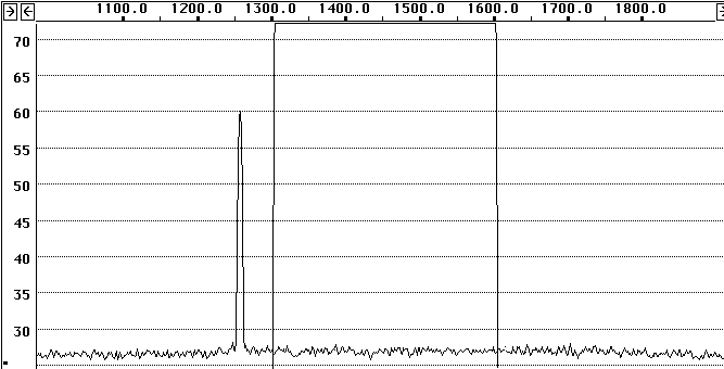
Fig. 3 The baseband spectrum of Linrad when doing NF measurements with a signal generator. The input signal is the audio from the same IC-706MKIIG as used in Fig. 2 when a –130dBm signal is applied to the input. Straight lines are drawn between the pixels to make the figure better visible in printing. The rectangular filter goes from 1300 to 1600 Hz.
7. CRYSTAL NOTCH FILTERS
Both DR2 and DR3 measurements are easy if one has signal generators that are much better than the receiver under test. The big problem is: how do we know? Standard signal generators are surely not good enough for serious work. One has to build something better – but how do we know it really works as intended?Crystal notch filters are the solution. Of course a crystal bandpass filter could also be used to improve the spectral purity of a signal generator, but that is practical for DR2 measurements only. One would need one filter for each strong generator for DR3 measurements, and one would then lose the essential flexibility to measure intermodulation at several frequency separations. Fig. 4 shows a basic crystal notch filter.
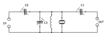
Fig. 4 The basic crystal notch filter. The coil and C3 form a parallel resonator which is selectively loaded by the crystal. C1 and C2 are equal. Smaller values for C1 and C2 gives deeper notches but the passband becomes narrower.
A parallel LC circuit is loaded by a crystal. The higher the impedance of the LC circuit is when not loaded by the crystal, the deeper is the notch. The LC circuit is a band pass filter. To get a high impedance at the same time as large bandwidth, one should use a large L/C ratio. This means keeping C3 small, so that the parallel capacitance of the crystal itself is the dominating capacitance. In practice it is also advantageous to do the impedance transformation inductively on the coil rather than using coupling capacitors as shown in Fig. 4 because that allows a larger L/C ratio and some more bandwidth.
If one wants to measure the dynamic range at close frequency separations, one does not only need a deep enough notch, one also needs it narrow - preferably 1dB or less attenuation at 5kHz away from the notch, with 30dB or more attenuation over a 1 kHz bandwidth at the notch center. This calls for more than one crystal.
Fig. 5 shows the schematic diagram of a practical notch filter for 14 MHz using three crystals. It is designed with very small tuning capacitors, to give the widest possible passband outside of the narrow notch.
The coils are wound on big toroids, Amidon T-80-6. This filter is intended for intermodulation measurements on 14 MHz and ideally the coils should be iron free. The 50 ohm windings are 13 turns and the tuned windings of the input and the output are 32 turns. The impedance that the crystals will load is thus 300 ohms. The toroids are heavily loaded by the input and the output, the loaded Q is low, and that is the reason the filter produces very low intermodulation despite the iron cores.
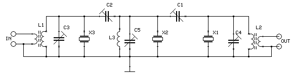
Fig. 5 A 14 MHz notch filter. C3 and C4 are 20pF trimmers tuned near the minimum capacitance. C1 and C2 are 60pF trimmers tuned to about 20pF. The inductors are wound on Amidon T80-6 toroids.
The frequency response of this notch filter is shown in Figs 6 and 7.
The layout of a notch filter like this is uncritical. Fig. 8 is a photograph how I made it. Tuning a filter like this is like tuning a bandpass filter with three LC resonators... not difficult at all if you have some kind of instrument to monitor the frequency response. Without any instruments at all it is possible to tune the filter for nearly zero attenuation 100kHz away from the notch. It will not be flat from 5 to 20 MHz automatically but it will certainly be flat enough to do dynamic range measurements.
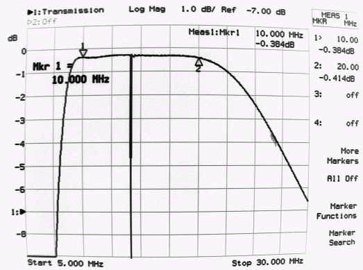
Fig. 6 Frequency response of filter in Fig 5 from 5 to 30 MHz. The filter attenuation is 0.3dB from 10 to 20 MHz.
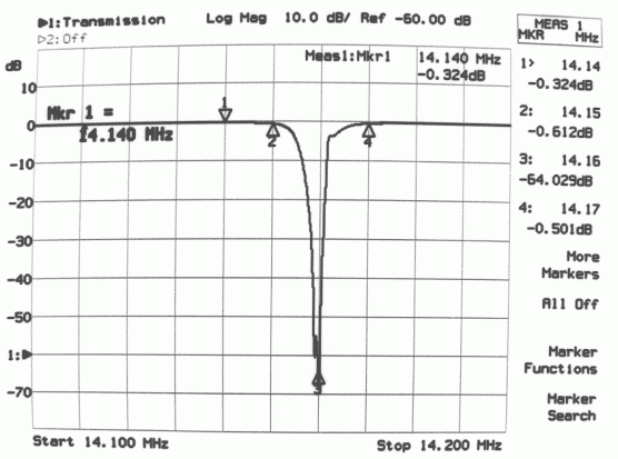
Fig. 7 Frequency response of filter in Fig 5 from 14.100 to 14.200 MHz. The filter attenuation is less than 0.5dB at 10kHz away from the notch, which is 50dB deep or more over 1.5 kHz.

Fig. 8 The 14 MHz notch filter built in a box made from double sided PCB material. The components are soldered to ground and the toroids are glued.
It is possible to design a 144 MHz filter the same way. The passband will be narrower and the notch wider because the parallel capacitance of the crystal gives a smaller L/C ratio and the series impedance at 144 MHz is not very low. The computer grade 16 MHz crystals I have used have a series impedance of about 300 ohms on the 9th overtone at 144.100 to 144.160 MHz. The overtone is not at the same place for different crystals, but buying 50 or 100 of these low cost devices makes it possible to get enough at the same frequency. Make sure that the crystals have a good 9th overtone resonance before buying many (some modern crystals are much smaller than the can suggests, and therefore may be useless at 144 MHz).
Fig. 9 shows a 144 MHz filter using eight crystals. It is basically the same configuration as shown in Fig. 5. This 144 MHz notch filter gives a 60dB deep notch. The frequency response is shown in Figs 10 and 11. A 16MHz crystal has false resonances above the main 9th overtone resonance. That gives rise to the spurious notches above the main notch in Fig. 11, so this kind of filter is not suitable to measure DR2 and DR3 with the undesired signals close to and above the desired signal.
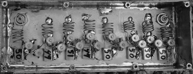
Fig. 9 A notch filter for 144 MHz. There is no iron, the impedance is stepped up by connecting the input and the output 1.5 turns from ground on coils having 4.5 turns.
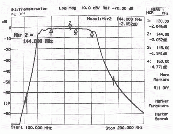
Fig. 10 Frequency response from 100 to 200 MHz of the notch filter shown in Fig. 9.
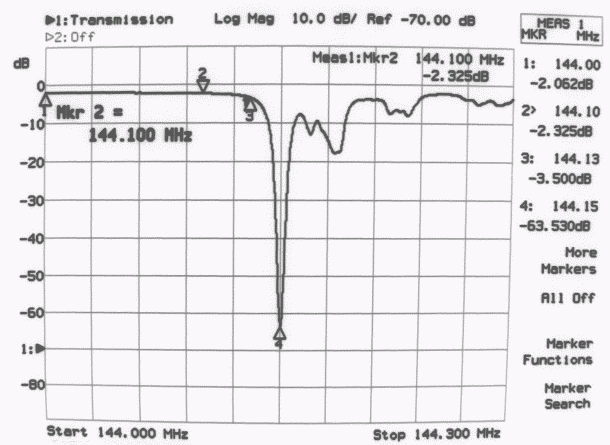
Fig. 11 Frequency response from 144.000 to 144.300 MHz of the notch filter shown in Fig. 9.
Also a crystal notch filter will produce third order intermodulation in DR3 measurements if the strong signals are close to the crystal resonance. At these frequencies the third order intermodulation products do not obey a third order law, even when the power level is far below the main signals, and amplifiers and mixers are behaving correctly. One has to go to very low power levels indeed to get true third order behaviour near the notch frequencies, and that is not so easy. To see it one has to use a very good receiver.
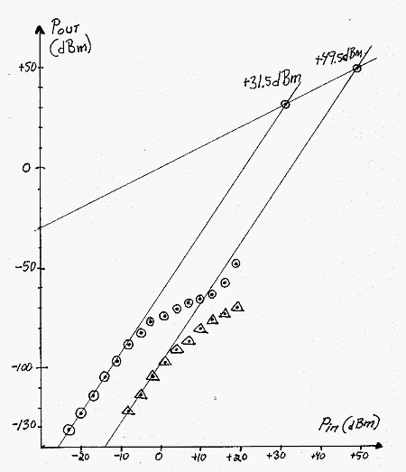
Fig 12 Signal levels at the output of a 144 MHz crystal notch filter in a two-tone test. Circles are for 20 kHz frequency separation, triangles for 100 kHz. The third order behaviour from very low levels is extrapolated towards the third order intercept points at +31.5 dBm for 20 kHz separation and at +49.5 dBm for 100 kHz separation. The intermodulation is created within the notch filter.
Fig. 12 shows the level of IM3 coming out from the 144 MHz notch filter at the notch frequency. The level of one of the two tones is also plotted for a 1:1 straight line. The two curves are measured at frequency separations of 20kHz and 100 kHz respectively. For this measurement 1W class A amplifiers followed by circulators were used in front of the combiner. The IM3 levels of the input signal to the notch filter are negligible. The notch filter was followed by an attenuator that was used to set the input to the RX144 converter well below the point where intermodulation is produced within the receive system. (The RX144 converter is the 144 MHz input of my high performance receiver hardware for Linrad. It is a quadruple frequency conversion radio with crystal oscillators only. The last conversion is from 2.5 MHz to DC, where a Delta44 soundcard converts wideband audio I and Q channels to digital form. (For details see http://antennspecialisten.se/~sm5bsz/linuxdsp/optrx.htm) The bandwidth was set to 3Hz and the Delta44 was run at maximum gain to achieve good sensitivity for the intermodulation products. It is quite clear from Fig. 12 that a crystal notch filter does not have the behaviour we are used to see in amplifiers and mixers. The third order behaviour which must be obeyed at very low signal levels stops already when the IM3 product is about 100dB below the level of the signal pair. The third order behaviour is extrapolated from low levels in Fig. 12: the third order intercept point for the notch filter is +31.5dBm for two signals separated by 20kHz, and +49.5dBm for two signals separated by 100kHz.
With two test signals at +16dBm the notch filter gives IM3 73dB below the signals so for normal amplifiers and mixers, IP3 values up to +45dBm can be measured accurately at 20 kHz separation at this power level. Without the notch filter the IM3 levels are at –74dBm allowing measurement up to IP3 values of about +55dBm but if the circulators are removed the IM3 is at –52dBm. Since the notch filter is needed anyway for the DR2 measurement it may be easier to use it than to make class A power amplifiers.
In summary, a crystal notch filter is a very practical piece of test equipment. It allows measurements to be done with standard laboratory signal generators which otherwise often are too noisy to allow evaluation of DR2. Measuring IM3 at the noise floor is difficult; a notch filter is one of the possible tools one can use, but the unusual behaviour of IM3 products must be remembered - especially when working close to the notch frequency.
8. PRACTICAL DETAILS OF DR2 MEASUREMENTS
For a conventional receiver, the level of the weak signal makes no difference as long as the dynamic range of the IF and audio sections of the receiver under test is adequate. It makes no difference at all if the AGC is enabled or not, if the spectrum analyzer at the loudspeaker output is being used to monitor the desired weak signal and the noise floor simultaneously.To check the dynamic range of the IF and audio sections, increase the level of the desired signal and monitor S/N. At some point S/N will no longer increase in proportion to the input level. This is the level where IF or audio noise is no longer small compared to the noise floor at the antenna input which has been reduced by AGC action or it is the level where the signal does not increase any more because of clipping. If the receiver under test has a dual loop AGC, the level where an RF attenuator is inserted will be clearly visible in the plot of S/N vs input power. DR2 measurements have to be made with the weak signal well below this level.
The way the two signal generators are combined is very uncritical for DR2. The power level needed for the strong signal is below 0dBm and the weak signal may be somewhere around –130dBm. A simple resistive network will be fine – connect the strong generator through a 5 ohm resistor and add the weak signal through a 500 ohm resistor. A directional coupler or even a T-connector followed by a 6dB pad to restore 50 ohms impedance will be fine.
For the measurement, just select a frequency offset and adjust the strong signal for a 3dB loss of S/N. DR2 is given by equation (3) above, where PGEN is the level of the strong signal at the antenna connector of the test object. If the signal generator is calibrated, one only has to subtract the loss due to the cables and the signal-combining network. If the generator is not calibrated (it could be a homemade low noise crystal oscillator) it is still possible to determine the power level from the noise figure as described in conjunction with Fig. 3 above, although one would then need calibrated attenuators to bring the power down for the saturation level to somewhere around –130 dBm. Signal leakage is the critical point here.
To give an idea about the significance of using a notch filter, Fig. 13 shows the screen of Linrad with the spectrum from 144.08 to 144.170 MHz when a HP8657A generator set to 144.0 MHz is connected through the notch filter. The data book says phase noise should be below –136dBc/Hz at a frequency separation of 20 kHz. The spectrum shown here shows that the sideband noise is –140dBc/Hz at a frequency separation of 100 kHz. State of the art commercial amateur transceivers are a little better than this, for example the TM255E tested at the Scandinavian VHF meeting in Gavelstad had a DR2 of 144.5dB at 100 kHz: http://antennspecialisten.se/~sm5bsz/dynrange/gavelstad/gav.htm
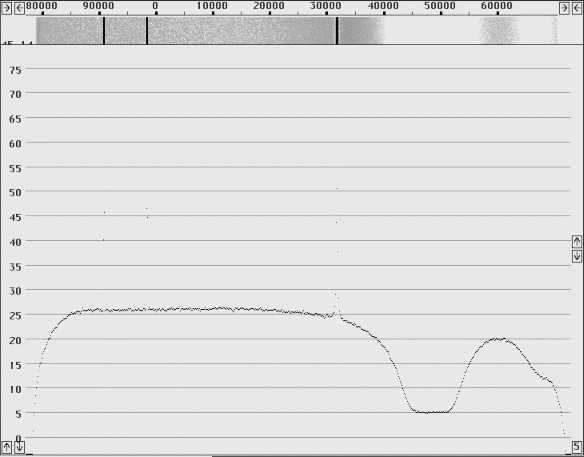
Fig 13 The Linrad spectrum of an HP8657A signal generator at 80 to 160 kHz offset. A practical illustration to the usefulness of a crystal notch filter for DR2 measurements.
9. PRACTICAL DETAILS OF DR3 MEASUREMENTS
Unlike the DR2 measurements, which do not really have any difficulties associated with them, DR3 measurements have all sorts of problems. It is very easy to come up with incorrect results, particularly if the measurements are made at low levels of the third order intermodulation products. On the other hand, measurements well above the noise floor may easily become incorrect if the S-meter or an RMS voltmeter at the loudspeaker output is used.By measuring DR3 with three signal generators as suggested here, it is possible to measure intermodulation correctly at high signal levels (but once again, if the unit under test has incorporated a dual-loop AGC, results will become incorrect at levels where RF gain is being reduced)
Problems with intermodulation measurement accuracy lie in the behaviour of the test receiver with strong intermodulating signals. One cannot trust the intermodulation to obey the third order law at high signal levels. For the more realistic situation with weak intermodulation products, below S6 or so, which we would typically notice when actually using the radio, the problems lie in intermodulation between the signal sources. These problems generally add some extra signal at the frequency where the third order intermodulation is expected. Typically one will therefore get results that underestimate the true performance of the tested unit, but the intermodulation signal could be in antiphase and then the error may go in the opposite direction.
Once a good source of two equally strong signals has been arranged (see more about that below), the rest of the DR3 measurement is easy. Use the block diagram of Fig. 2, and replace the noise generator with the two-signal source. Set the weak signal generator (the one injected through the directional coupler) to a frequency close to the frequency where third order intermodulation is expected. Set the two high-level generators for equal levels and then set the weak signal to have the same level as the intermodulation product as seen on the spectrum analyzer. It does not matter if AGC is on or off – one will easily see when the signals have the same amplitude. It does not even matter if AF stages become saturated. Even IF stages may be saturated, provided that the two interfering signals are outside the IF passband. When intermodulation is measured this way, the third order law is confirmed over a much larger range of input signal levels than one typically observes with other methods.
Fig. 14 shows the levels of third order intermodulation in an IC-706MKIIG at input levels in the range –56 to –8dBm. As one can see from the measured data, third order intermodulation shows accurate third order behaviour up to a point when it is about 40dB below the two tones. To make this measurement a nearly perfect two-tone generator was used. With the aid of the RX144 and Linrad the source was verified to have IM3 far below the levels recorded for the IC-706MKIIG. It is of course essential that the source of the weak signal is very well screened. Any leakage will cause incorrect results at low levels of IM3.
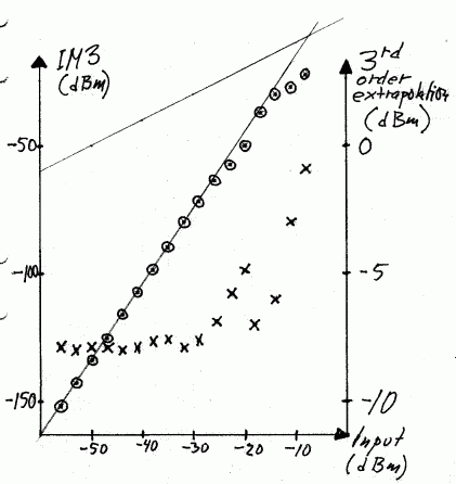
Fig 14 Measured levels of third order intermodulation (circles) for an IC-706MKIIG with RF amplifier off and with AGC enabled. The result of a third-order extrapolation (crosses) gives the correct result (IP3= –8 dBm) up to IM3 levels that are about 40dB below the main signals.
The following sub-sections identify problem areas that need attention when combining two high level signal generators to make a two-tone source for DR3 measurements.
Signal generator harmonics
First of all the two signal generators that are to be combined have to be free of harmonics. If for example two generators at 144.100 and 144.125 are used, the third order intermodulation products are expected at 144.075 and 144.150 MHz respectively. If both generators have some signal at the second harmonic, difference frequencies 288.250 -144.100 = 144.150 and 288.200 – 144.125 = 144.075 may be generated. The frequencies are exactly where the third order intermodulation products will appear. Even worse, these difference frequencies are second order so they do not fall off as rapidly as the third order products. Therefore the second order products related to generator overtones may dominate at low levels of intermodulation. To get an idea of what the consequences are, look at Fig. 15, which is a plot of the output from a wideband amplifier using BFR91A. Linrad with RX144 is used as a spectrum analyzer. The signal level and the levels at the two IM3 frequencies are measured directly with the Linrad S-meter. The input signal ranges from –29dBm to –59dBm. For these measurements the signal generators were followed by deliberately saturated amplifiers that produced second harmonics about 25dB below the main signals. At such a high harmonic content into a wideband amplifier, it is not surprising that the deviations from normal third order behaviour is rather large. For a comparison, Fig. 15 also shows data measured with a bandpass filter for 144 MHz inserted in the same setup to reduce the harmonics to about –75dBc.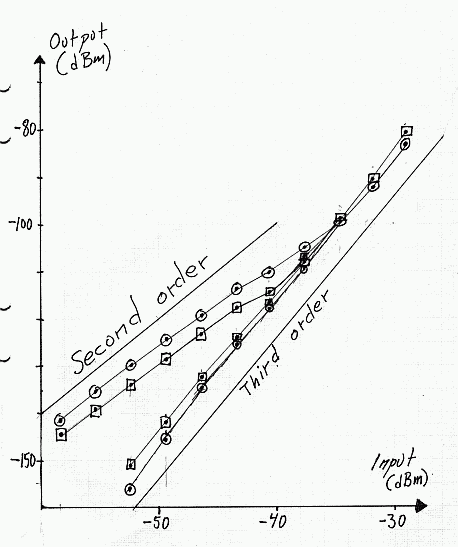
Fig 15 IM3 measurements on a BFR91A wideband amplifier. The upper (circles) and the lower (boxes) intermodulation frequency signal level with and without a filter that removes the second harmonics from the test signal. Note that presence of harmonics causes a second order behaviour at low levels.
The wideband amplifier used to produce Fig. 15 has IP3 at about –4 dBm. It must be measured with input signals above –38 dBm when the harmonics are at –25dBc. The third order intermodulation products are then at about –107 dBm which is about 40 dB above the noise in 2 kHz bandwidth. Trying to measure the third order intermodulation free dynamic range at the noise floor would give incorrect results. Second harmonics of the test signals will often be suppressed by the input filters of the test receiver, but it is still a good idea to make sure the test signals are not polluted with harmonics, particularly if external amplifiers are used to raise the power level. More power makes it easier to combine two signals without intermodulation, but simple saturated amplifiers need lowpass or bandpass filters at the output. If the144 MHz notch filter described above is being used to remove noise sidebands, it also provides very good harmonic suppression at 288MHz and above.
Mutual intermodulation between generators
The two strong signals required for a DR3 measurement are usually obtained by the arrangement shown in Fig.16.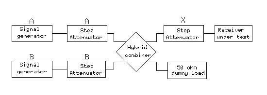
Fig 16 Two signal generators are combined and isolated from each other with a hybrid combiner. See text. A suitable hybrid combiner can be made from coaxial cable. Avoid ferrite transformers – they may produce intermodulation. An iron-free hybrid combiner with built-in dummy load can also be made with coils, capacitors and a resistor. The hybrid will isolate the inputs from each other by something like 30 or 40dB if both outputs are terminated in 50 ohms. Note that the receiver under test is actually not likely to have an input impedance of 50 ohms – although it is designed for good noise figure and intermodulation characteristics when the source impedance is 50 ohms, this does not imply that the input impedance is 50 ohms. The input impedance of the IC-706MKIIG that I use as a reference for a typical modern rig has an input impedance at 145MHz of 55 ohms and 18pF. The input VSWR is 3.0 and the return loss is -6dB. If such a receiver is connected directly to the hybrid, even a perfect hybrid will degrade the isolation between the generators to only 12dB. For each dB of attenuation in front of the receiver under test, the isolation will improve by 2dB until the isolation reaches 25dB or so. The hybrid simply works as a VSWR bridge and it measures the reflected wave from the receiver under test. 50% of the power from generator A goes to the dummy load, 50% goes to the test port, comes back as a reflected wave and is then split equally into generator A and B that receive 25% each. Therefore the reflected wave minus 6dB is all the isolation one can get. For a given level of the test signal into the receiver it does not matter if attenuation is made in front of the hybrid or after the hybrid, as long as the isolation provided by the hybrid is far from the limit.
When the output attenuator is set high enough, small impedance errors may cause large changes of the near zero coupling between the generators. By fine-tuning the impedance of the dummy load it is possible to cancel the coupling completely, but only from A to B or vice versa. The reason is that balancing is frequency dependent, but if the two generators are very close spaced balancing is a way of removing mutual intermodulation in the generators at high signal levels.
With good generators such as the HP8657A, worst case intermodulation levels for the configuration of Fig. 16 are shown in Fig. 17. The figure shows measured intermodulation levels at different power levels into the test object which is the same impedance as the IC-706MKIIG. The attenuator X is set to 3dB and the attenuators A and B are the attenuators built into the generators. To make accurate measurements of low intermodulation levels a directional coupler is inserted between generator A and the hybrid for the data in Fig. 17.
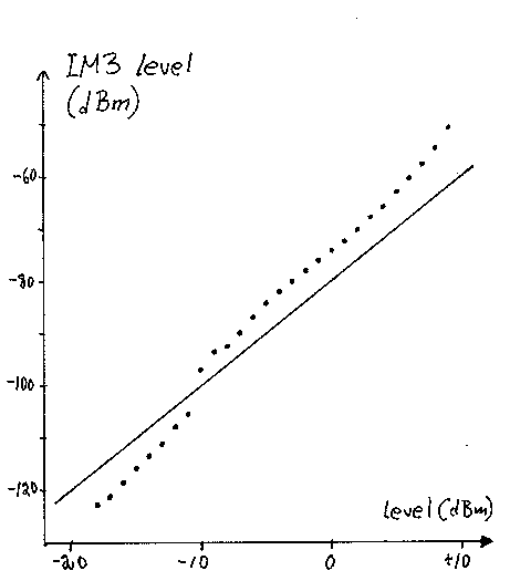
Fig. 17 The intermodulation produced in a HP8657A when used for a two-tone test. The discontinuity between –10 and –11dBm is between –3dBm and –4dBm power output from the signal generators. It is due to the internal architecture of the HP8657A generator.
To generate an IMD product at the noise floor in SSB bandwidth, the IM3 product will need to be at about –130dBm if a noise figure of about 10dB is assumed. This calls for IM3 levels from the generator of less than –140dBm. Extrapolating from Fig. 17, one finds that the maximum signal level one may use is then about –30dBm. This means that a pair of HP8657A generators can be used for IM3 measurements at the noise floor up to a third order intercept point of about +20dBm. An old vacuum tube free-running oscillator, the HP608D produces 12dB more intermodulation than the HP8657A if it is properly calibrated. However, by turning the output level control to maximum one can get +13dBm output power rather than the +4dBm that is the maximum when the control is “properly” set. This means that 9dB more attenuation can be used and then the HP608D becomes better than the HP8657A, with IM3 about 7dB lower.
It is a good idea to check what really comes out from the signal generators, by use of a directional coupler. If you do not have a good enough spectrum analyzer (RX144 + Linrad) you can use the receiver that will later become the test object. The signal extracted from a directional coupler will have the signal from the other generator suppressed by something like 20dB but the IM3 product will be present on the opposite side in frequency and its level below the generator signal is the same as will be presented to the test object in the real test. In this case the test object will produce at least 20dB less IM3 since it is not loaded by equal signal levels at the two frequencies due to the directional coupler. With a second directional coupler and a third generator one can measure the levels of signal and IM3 and make sure that the IM3 produced by the generator is well below the IM3 produced by the test object. Do not forget to allow the hybrid to see the same impedance as it will see later when the test object is connected to it. An open 3dB pad will correspond to VSWR=3 and may be used in the test port of the hybrid. Leave this 3dB pad in place and connect the test object after it to ensure the generator intermodulation will be smaller than the value you have checked.
It has been suggested that one can distribute the attenuation differently between attenuators in front of and after the hybrid to find out if there is a problem with IM3 produced in the generators. The idea is that the isolation provided by the hybrid will be constant and that therefore the attenuators in front of the hybrid will affect the intermodulation produced in the generators while the attenuator after the hybrid will not. This might be the case sometimes, but it will certainly not be true for a test object with an unmatched input, such as almost any low-noise VHF receiver.
To illustrate the effect of generator intermodulation, I have measured the IM3 levels of the IC-706MkIIG with two HP8657A generators set to +10dBm connected directly to the hybrid. The test port of the hybrid is connected to a step attenuator and also loaded by 18pF to make the hybrid see VSWR=3. The step attenuator is used to set the level of the test signal pair. The maximum available power level is +4dBm. Fig. 18 shows the result. As expected, the intermodulation shows first order behaviour at low signal levels where the intermodulation produced in the generators dominates.
This measurement is intended to show a way of making an incorrect measurement, and what the result might look like. Fig. 18 is an extreme case of poor measurement engineering, where only the output attenuator is used to set the signal level. Obviously the mismatch at the hybrid output will be much smaller in a real measurement; the 18pF capacitance provokes a really bad VSWR. It is convenient to set the level of both generators simultaneously on the output attenuator X in Fig. 16; but as soon as one reaches the point where isolation does not improve by the full return loss improvement (typically at an attenuation in the order of 10dB or less), it is much better to use the attenuators at the generator side.
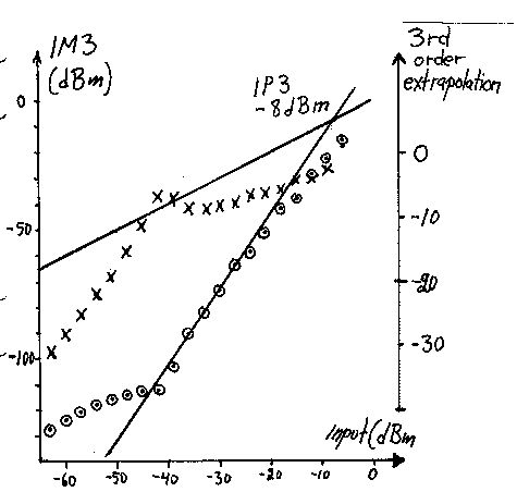
Fig 18 Measured level of third order intermodulation, (circles), for an IC-706MKIIG with RF amplifier off and with AGC enabled. This is the same measurement as in Fig.14 but with poor isolation between generators. The formula for evaluating IP3, result (crosses) gives the correct result (IP3 = –8dBm) in a narrow range only. At low levels the intermodulation in the generators dominates and at high levels the receiver under test does not have third order behaviour.
If measurements are done without the aid of an audio spectrum analyzer, all sorts of further errors are possible. If modern (synthesized) generators are used, they are likely to have spurs every 10kHz and/or every 100 kHz. Fig. 19 shows the waterfall graph recorded from two HP8657A generators delivering –15dBm into the RX144. The lower part of the image shows IM3 only, but the upper part of the image shows all the noise and spurs that became visible without the notch filter which was used for the lower half. The loss of the filter was compensated for, so the level of the two strong signals was the same in both cases. Note the strong spurs 100 and 200 Hz below the intermodulation product. The generators, 100 kHz separated in frequency were offset by 100 and 200 Hz to move the spurs away from the IM3 frequency. One has to check for these spurs by running one generator only, because each strong spur belongs to one generator only. The notch filter removes spurs and lowers the noise floor so it makes IM3 stand out clearly even at low IM3 levels. Note that IP3 is not exceptional for the RX144; it is only about +25dBm, a level that is not difficult to reach taking the system noise figure of about 16dB into account. A narrowband receiver is easily much better than this; measuring IP3 near the noise floor may be really difficult on top performance receivers. If a third generator is not used, measuring IM3 well above the noise floor may be really difficult too.
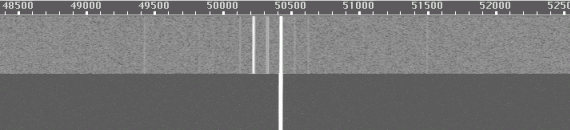
Fig. 19 Two HP8657A generators at 143.9498 and 144.0499 produce IM3 at 144.1500 MHz (there is a calibration error of 430Hz). The lower half of this waterfall graph is with the composite test signal through a notch filter. Only IM3 is visible. The upper half is without notch filter: spurs and sideband noise are not much below the IM3 product at –82dBc. The HP8657A generators are not suitable to measure IM3 lower than about –70dBc without a spectrum analyzer and not lower than about –90dBc without a notch filter.
When class A power amplifiers are used to allow measurement at the noise floor of very good receivers, one has to be extra careful with screening. Doubly shielded coaxial cables and good connectors are needed to make sure there is no leakage causing intermodulation in the amplifiers. One also has to make sure connectors are clean and of good quality, because intermodulation may be produced in poor connections, switches of stepped attenuators and elsewhere.
10. HOW MUCH DR DO WE NEED?
Based on surveys of actual signal levels at 7MHz, Peter Chadwick, G3RZP [11] arrived at the conclusion that PNDR (Phase Noise Limited Dynamic Range) should be at least 100dB and that ILDR (Intermodulation-limited dynamic range) should be at least 96dB.These numbers refer to an SSB bandwidth, and in the terminology I have used in this article it means DR2 should be at least 133dBHz and DR3 should be at least 129dBHz.
On the VHF bands, the basic principles remain exactly the same but the numbers are different. The needs will also vary much more at different locations. There are two kinds of problems: out-of-band interference and in-band interference. The out-of-band interference is typically at a large frequency separation, mainly FM and TV broadcast stations with very high ERP powers. This is a problem for a preamplifier and filters associated with it. In-band interference from our fellow amateurs can not easily be taken care of with filters, so here we need a good radio with high dynamic range.
On 144 MHz amateurs typically produce power levels of 3kW ERP with 100W RF into a 13dBd antenna, but ERPs of 100kW are also not uncommon – 1kW into 4 modest yagis with 18dBd array gain. The received powers at some different distances are given in Table 3 under the assumption of free space propagation.
|
Distance |
Tx ERP |
Rx Ant = |
Rx Ant = |
|
1 |
3 |
+2.4 |
+7.4 |
|
1 |
100 |
+17.4 |
+22.4 |
|
10 |
3 |
-17.6 |
-12.6 |
|
10 |
100 |
-2.6 |
+2.4 |
In reality we do not have free space conditions. Reflections from ground change the signal level in an unpredictable way because the ground is typically not flat at all. Nevertheless Table 3 indicates that a rig capable of dealing with –20dBm power from neighbouring amateurs would be useful at some locations. This translates to a DR2 of 154dBHz, which is possible but nothing one can expect from standard transceivers today. Table 3 also shows that for two EME-grade stations at a distance of 1km to work undisturbed with antennas pointing into each other, they would need a DR2 of about 200dB! That is impossible today and will most probably remain impossible.
Worst case in-band interference at VHF is typically dominated by a single signal. It happens when you have your main lobe pointing towards the nearest neighbour while he is pointing in your direction. Contrary to the situation on the HF bands, the DR2 requirements on VHF may therefore be far more stringent than the DR3 requirements.
When testing receivers, one has to collect and present a large amount of data. It is relevant to measure DR2 at several frequency separations, and a reasonable choice is 5, 20, 100 and 500kHz. It would probably be enough to measure DR3 at 5, 20 and 100 kHz separation, but still the amount of data is much larger than what is commonly published in product testing.
On the other hand, there is no reason to measure everything with and without preamplifier because the influence of a preamplifier should be easy to see – a preamp lowers IP3 by the amount of gain it has; and it reduces DR3 by an amount given by the preamp gain minus the improvement in the noise figure. DR2 should be affected only if it is limited by blocking, something that is uncommon in modern receivers. Within the limitations of available page space for reviews, it would be a good idea to focus product testing on the performance without the preamplifier, and simply specify the gain and noise figure improvement obtainable by switching in the preamplifier. Additional measurements can always be posted on the web (which is already ARRL’s practice).
At VHF/UHF, an analysis of gain and dynamic range performance will show that it is always better to use a mast-mounted preamplifier, and to operate the main receiver with its built-in preamplifier switched off. A serious VHF/UHF weak signal enthusiast will always do this, so this is another reason for equipment reviews to focus mainly on the VHF/UHF performance data obtainable without the preamplifier. The noise from that preamplifier (including amplified antenna noise) should be the dominating contribution to the noise floor of the entire system. As a consequence signal levels are raised by something like 15 dB, and this is another reason why dynamic range requirements are much harder to meet at VHF/UHF, compared to HF bands where usually no preamplifier is needed.
References
[1] Ulrich L. Rohde, Theory of Intermodulation and Reciprocal Mixing: Practise, Definitions and Measurements in Devices and Systems, Part 2 QEX Jan/Feb 2003 p. 21-31.[2] Ed Hare, W1RFI, Swept Receiver Dynamic Range Testing in the ARRL Laboratory. QEX June 1996 p. 3.
[3] http://www.w8ji.com/receivers.htm
[4] http://nlrs.dropboxone.net/Aurora-2002/W0ZQ/ReceiverDynamics.doc
[5] http://qrp.kd4ab.org/2001/010112/0049.html
[6] http://www.kachina-az.com/an108.htm
[7] http://www.natworld.com/ars/pages/lab_text/notes_bdr.html
[8] http://nlrs.dropboxone.net/Aurora-2002/W0ZQ/ReceiverDynamics.doc
[9] J. W. Healy, NJ2L, Kenwood TS-450S and TS-690S Transceivers QST, April 1992, p. 67-71.
[10] R Bertelsmeier, DJ9BV, Myths and Facts about Preamp Tuning DUBUS Technik V, 1998, p. 150-158.
[11] Peter E Chadwick, G3RZP, HF Receiver Dynamic Range: How Much Do We Need? QEX May/June 2002, p 36-41.